Blue Q boxes are questions for you to answer by hand, in a notebook, with a pen. Not because I am old fashioned. Writing something down by hand is slow, and slow is the point: it is very hard to write an explanation you do not actually understand. You are welcome to use AI in this class for the mechanics of code, but these boxes are the part where you do the thinking yourself. Bring your written notes to class, I will ask to see them.
Green You Try boxes are optional code for you to work through. Nothing is collected and nothing is graded. They are there because you will learn more from changing a number and rerunning than from watching me do it.
Every code cell begins with a tag that tells you what to do with it.
# RUN THIS. Setup, loading data, a plot. Copy it, run it, move on. You do not need to be able to write it from memory.
# LEARN TO WRITE THIS. The pattern of the day. The homework will ask you for it, and so will the exam. Type it out yourself at least once rather than pasting it.
# DEMO ONLY. Fake data or a contrived experiment that exists to show one idea. You would never write this for a real project and you do not need to be able to.
Short answers to the Q boxes are in drop down boxes at the very bottom. Write yours first.
Reading: You have not met decision trees yet, so start with Geron chapter 5, the sections Training and Visualizing a Decision Tree, Making Predictions, Regularization Hyperparameters, and Decision Trees Have High Variance. Then chapter 6, the sections on Voting Classifiers, Bagging and Pasting, and Random Forests.
Welcome to Unit 2! On Day 5 our logistic regression found good wines with an average precision of 0.532 on the validation set. Today we beat that, and we do it with a strange idea: take a model that is pretty bad on its own, make hundreds of copies of it, and let them vote.
The model we make copies of is a decision tree. Most of you have not met decision trees yet (DATA 201 gets to them later this semester), so the first part of today is a quick introduction. Then we let the tree grow too big and watch it fall apart, and then we fix it!
We are using the same wine data and the exact same split as Day 5, so every number today can be compared to Day 5.
Setup and the Same Split as Day 5
Same data, same good column, same two splits with the same random_state. The test set gets put away again. Everything until the section called “The Test Set, Once” happens on the validation set.
# RUN THIS. The Day 5 wine and the Day 5 splits, exactly.import numpy as npimport pandas as pdimport matplotlib.pyplot as pltfrom sklearn.model_selection import train_test_splitwine = pd.read_csv("data/winequality-red.csv", sep=";") # this file uses semicolons, not commaswine["good"] = (wine["quality"] >=7).astype(int) # 1 if quality is 7 or 8, 0 if notX = wine.drop(columns=["quality", "good"])y = wine["good"]# split the test set off first and put it awayX_train_full, X_test, y_train_full, y_test = train_test_split( X, y, test_size=0.25, stratify=y, random_state=42)# split a validation set off the training dataX_train, X_valid, y_train, y_valid = train_test_split( X_train_full, y_train_full, test_size=0.25, stratify=y_train_full, random_state=42)print("training rows: ", X_train.shape[0])print("validation rows:", X_valid.shape[0])print("test rows: ", X_test.shape[0], " (put away)")
training rows:   899
validation rows: 300
test rows:       400   (put away)
One thing is missing on purpose: there is no StandardScaler today. You will see why in a minute.
Decision Trees - an Overview
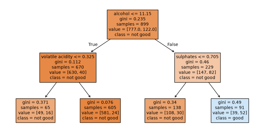
A decision tree makes a prediction by asking a short list of yes or no questions, one feature at a time. Is the alcohol above 11.15? If yes, are the sulphates above 0.705? Every wine starts at the top, answers the questions, and ends up in a box at the bottom called a leaf. The prediction is whatever most of the training wines in that leaf were.
Where do the questions come from? The tree picks them. At each step it tries every feature and every cutoff, and keeps the one question that best separates good wines from not good wines. Then it does the same thing again inside each half. You do not choose the questions, the data does.
Let’s grow a tiny one, only two questions deep, so we can read the whole thing.
# LEARN TO WRITE THIS. A small decision tree.# You will see this again in Data201!from sklearn.tree import DecisionTreeClassifiertree_small = DecisionTreeClassifier( max_depth=2, # at most two questions in a row, then stop random_state=42) # ties between equally good questions are broken at random, this fixes ittree_small.fit(X_train, y_train)
In a Jupyter environment, please rerun this cell to show the HTML representation or trust the notebook. On GitHub, the HTML representation is unable to render, please try loading this page with nbviewer.org.
# RUN THIS. Draw the tree.from sklearn.tree import plot_treeplt.figure(figsize=(11, 5.5))plot_tree(tree_small, feature_names=list(X.columns), # so the boxes say "alcohol" instead of "x[10]" class_names=["not good", "good"], # class 0 first, then class 1 filled=True, # color the boxes: orange leans not good, blue leans good precision=3, # show cutoffs to 3 decimal places fontsize=10)plt.savefig("images/01-small-tree.png", dpi=150, bbox_inches="tight")plt.show()
Since we set max_depth = 2 we see that our tree branches two times giving us three layers if we count the top box.
Here is how to read one box.
The first line is the question. Wines that answer yes go left (the arrow says True), wines that answer no go right.
samples is how many training wines landed in this box.
value is how many of them were [not good, good], in that order.
class is the majority, and it is what the tree predicts for any wine that ends in this box.
gini measures how mixed the box is. 0 means every wine in the box is the same class. You can ignore it for today.
The top box has all 899 training wines, 777 not good and 122 good. The first question the tree chose is about alcohol. So in the second row we see that 670 wines had alcohol below or equal to 11.15 and 229 had alcohol above. Next we tested on sulphates along one branch and volatile acidity on the other. If we look along the bottom row. The box with 605 wines (lower alcohol, higher volatile acidity) has only 24 good wines in it, about 4 percent. The box on the far right (higher alcohol, higher sulphates) is the only one where good wines are the majority: 52 of 91.
A tree can give probabilities too. For a wine that lands in that far right blue leaf, predict_proba says 52 / (39+52) = 52 / 91 = 0.571 good. It is just the share of good training wines in the leaf.
Why did we skip StandardScaler in this case?!? Every question compares one feature to a cutoff. Whether alcohol is measured in percent or in parts per million, “is it above the cutoff” gives the same answer for every wine. Trees do not care about scale or units of a variable, so we do not scale.
Q1. Write this one out by hand
a. A new wine has alcohol 12.1, volatile acidity 0.40, and sulphates 0.80. Trace it through the tree. Which leaf does it land in, what does the tree predict, and what probability of good does it give?
b. A second wine has alcohol 9.8 and volatile acidity 0.60. Which leaf does it land in? Why did the tree never ask about its sulphates?
c. Explain in your own words why a decision tree does not need scaled features, but logistic regression did.
Let the Tree Grow
Two questions is a pretty crude model. What if we let the tree ask as many questions as it wants? With no max_depth, the tree keeps splitting until every leaf is pure, meaning every training wine in it is the same class.
# LEARN TO WRITE THIS. A tree with no limit, # This time scored on training and on validation.from sklearn.metrics import accuracy_score, average_precision_score# Choose and train the modeltree_big = DecisionTreeClassifier(random_state=42) # no max_depth, so it grows until every leaf is puretree_big.fit(X_train, y_train)# Notice the tree_big. has lots of variables, use tab complete to see them all!# Show the depth and number of leavesprint("depth:", tree_big.get_depth(), " leaves:", tree_big.get_n_leaves())# how well does it do on the wines it trained on?# Get the accuracy score by sending in the real training data and the predicted datatrain_acc = accuracy_score(y_train, tree_big.predict(X_train))print("training accuracy:", round(train_acc, 3))# Don't forget you also have a validation set that was not used during training# and on the validation wines, using the Day 5 score for rare positivesy_prob_tree = tree_big.predict_proba(X_valid)[:, 1]print("validation average precision:", round(average_precision_score(y_valid, y_prob_tree), 3))
depth: 12    leaves: 95
training accuracy: 1.0
validation average precision: 0.299
The tree asked questions 12 deep and made 95 leaves. It got every single training wine right, a training accuracy of 1.0. On validation its average precision is 0.299. We are perfect on the training data and not great on the validation data…. classic overfitting!
You have seen this before. It is the degree 15 polynomial from Day 2. The tree memorized the training wines, including all their noise, and what it memorized does not carry over to new wine. In Day 3’s language, a fully grown tree has low bias and very high variance.
Below we train five trees, and each one sees a slightly different version of the training data. (How we make those versions is called a bootstrap sample, and it is the key idea of the Bagging section. For now just watch the scores.)
# DEMO ONLY. Five trees, each trained on a slightly different copy of the training data.# The loop walks over five random seeds. Each seed gives a different resampled copy.for seed in [0, 1, 2, 3, 4]: X_boot = X_train.sample(frac=1, replace=True, random_state=seed) # resample the rows, explained below y_boot = y_train.loc[X_boot.index] # the labels that go with those rows tree = DecisionTreeClassifier(random_state=42) tree.fit(X_boot, y_boot) ap = average_precision_score(y_valid, tree.predict_proba(X_valid)[:, 1])print("seed", seed, " validation average precision:", round(ap, 3))
seed 0   validation average precision: 0.367
seed 1   validation average precision: 0.213
seed 2   validation average precision: 0.245
seed 3   validation average precision: 0.261
seed 4   validation average precision: 0.274
NOTICE - Each time we sampled just slightly different data (here we randomly picked data points allowing some to be seen more than once and others not at all) we got different average precision. Recall from last class the average precision score is roughly the area under the precision recall curve.
What do we see here? Same kind of model, nearly the same data, and the score swings from 0.213 to 0.367. That is what high variance means in practice: small changes to the training data make big changes to the model. We should not trust this decision tree model.
So we either need to regularize (prune the tree - we talk about this in Data 201 and you can think about other things suggested in the reading) or we need to come up with a way to force the decision tree to make better decisions rather than memorizing.
Q2. Write this one out by hand
a. The big tree got a training accuracy of 1.0. Why is that a warning sign rather than good news? Connect it to something from Day 2 or Day 3.
b. Name two settings you could use to stop a tree from growing so big. (max_depth is one. Geron chapter 5, Regularization Hyperparameters, lists others.)
c. The five trees above got validation scores between about 0.21 and 0.37. If you had to pick one of them, how would you choose, and why should that choice make you nervous?
Let’s Crowd Source!
Here is the idea the rest of today is built on. Suppose you have a lot of models that are each only a little better than guessing, and you let them vote. If their mistakes are independent (they do not all get fooled by the same wines), the majority can be right much more often than any one voter.
This is easier to see with fake data than with wine. Below, every voter is right 51 percent of the time, barely better than a coin flip. We ask 2000 questions and check how often the majority is right.
# DEMO ONLY. Voters who are each right 51 percent of the time, voting on 2000 questions.# Just making fake random data hererng = np.random.default_rng(42)for n_voters in [1, 11, 101, 1001]: votes = rng.random((2000, n_voters)) <0.51# True means that voter got that question right right_votes = votes.sum(axis=1) # how many voters got each question right, add up the ones majority_right = right_votes > n_voters /2# did more than half of them get it right?print(n_voters, "voters: the majority is right", round(majority_right.mean(), 3), "of the time")
1 voters: the majority is right 0.514 of the time
11 voters: the majority is right 0.518 of the time
101 voters: the majority is right 0.584 of the time
1001 voters: the majority is right 0.756 of the time
Notice how as we increase the number of voters the majority answer is right more of the time.
One voter is right about half the time. But with 1001 voters the majority is right 0.756 of the time. Nobody got smarter. The mistakes just cancel out.
The catch is the word independent. These fake voters each flip their own coin. Real models trained on the same data tend to make the same mistakes, and then voting does not help much. So if we want a crowd that actually helps, we need voters that make different mistakes. The next two sections are two ways to manufacture that.
Q3. Write this one out by hand
a. In the fake voting example, why did the majority get so much better as we added voters? What assumption about the voters made that happen?
Bagging
Bagging (short for bootstrap aggregating). The goal is to force the crowd to be different on purpose. Instead of training every tree on the same data, it trains each tree on its own bootstrap sample.
A bootstrap sample is made by drawing rows from the training set with replacement until you have as many rows as you started with. With replacement means a row can be picked more than once, and some rows never get picked at all. Here is an example
# RUN THIS. One bootstrap sample of the 899 training wines.X_boot = X_train.sample( frac=1, # draw as many rows as we started with replace=True, # a row can be picked again. This is what makes it a bootstrap sample random_state=42)print("rows in the bootstrap sample:", len(X_boot))print("different wines in it: ", X_boot.index.nunique())print("share of the training wines that made it in:", round(X_boot.index.nunique() /len(X_train), 3))
rows in the bootstrap sample: 899
different wines in it:        552
share of the training wines that made it in: 0.614
899 rows in the data (same as the training set), but only 552 different wines, about 61 percent of them. Some wines are in there two or three times and the rest are missing. (On big data this settles at about 63 percent, and Geron explains why in the Bagging and Pasting section.) Every tree gets its own bootstrap sample, so every tree sees a different mix of wines, grows different questions, and makes different mistakes. Then they vote by averaging their probabilities.
If you draw without replacement instead, it is called pasting. Bagging is the one you will actually see used.
# LEARN TO WRITE THIS. 200 trees, each on its own bootstrap sample, averaged.from sklearn.ensemble import BaggingClassifier# Create the modelbag = BaggingClassifier( DecisionTreeClassifier(), # the model to make copies of n_estimators=200, # how many copies of the model to make, each on its own bootstrap sample random_state=42)# Train the modelbag.fit(X_train, y_train)# Get the probabilitiesy_prob_bag = bag.predict_proba(X_valid)[:, 1]print("bagging, validation average precision:", round(average_precision_score(y_valid, y_prob_bag), 3))
bagging, validation average precision: 0.641
0.641. Each of those 200 trees is a fully grown, badly overfit tree like the 0.299 one. Averaged together they beat logistic regression by a lot. Each tree memorized different noise, and when you average them the noise mostly cancels while the real pattern (the part they all agree on) survives.
Q4. Write this one out by hand
a. In your own words, what is a bootstrap sample? Why does it matter that it is drawn with replacement?
b. A single fully grown tree scored 0.299. 200 of them bagged together scored 0.641. Each tree is just as overfit as before. So where did the improvement come from?
c. Bagging reduces variance. Look back at Day 3: is the big tree’s problem bias or variance? Would bagging help a model whose problem was bias?
Random Forests
A random forest is bagging with one more trick. When a tree is choosing its next question, it is only allowed to look at a random handful of the features, a different handful at every question. With 11 wine features, sklearn’s default lets each question choose from 3 of them (the square root of 11, rounded down).
Why would you make each tree worse on purpose? Because in plain bagging, every tree still tends to ask about alcohol first (all five of our resampled trees did). The trees end up similar, and similar trees make similar mistakes. Hiding alcohol from some of the questions forces the trees to find other ways to spot a good wine, so they disagree more, and the vote gets better.
# LEARN TO WRITE THIS. A random forest.from sklearn.ensemble import RandomForestClassifierforest = RandomForestClassifier( n_estimators=200, # number of trees max_features="sqrt", # each question looks at a random sqrt(11), so 3, of the features. This is the default random_state=42) # the bootstrap samples and feature choices are random, this makes them repeatableforest.fit(X_train, y_train)train_acc = accuracy_score(y_train, forest.predict(X_train))y_prob_forest = forest.predict_proba(X_valid)[:, 1]print("training accuracy:", round(train_acc, 3))print("validation average precision:", round(average_precision_score(y_valid, y_prob_forest), 3))
training accuracy: 1.0
validation average precision: 0.667
Validation average precision 0.667, the best so far. Notice the training accuracy is still 1.0. Every tree in the forest is still overfit! In a forest that is fine, and it is the one place in this class where perfect training accuracy is not a red flag. The individual trees overfit in different directions, and the average does not.
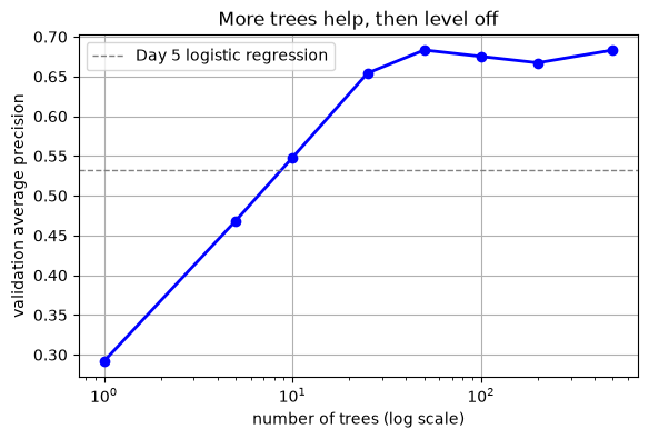
How many trees do you need? More trees never make a forest worse, they only make it slower. Here is what happens as we add them.
# RUN THIS. Validation average precision as the forest grows.tree_counts = [1, 5, 10, 25, 50, 100, 200, 500]scores = []for n in tree_counts: f = RandomForestClassifier(n_estimators=n, random_state=42) f.fit(X_train, y_train) scores.append(average_precision_score(y_valid, f.predict_proba(X_valid)[:, 1]))print(np.round(scores, 3))plt.figure(figsize=(6.5, 4))plt.semilogx(tree_counts, scores, "bo-", linewidth=2)plt.axhline(0.532, color="gray", linestyle="--", linewidth=1, label="Day 5 logistic regression")plt.xlabel("number of trees (log scale)")plt.ylabel("validation average precision")plt.title("More trees help, then level off")plt.grid()plt.legend()plt.savefig("images/02-trees-vs-ap.png", dpi=150, bbox_inches="tight")plt.show()
[0.292 0.469 0.548 0.654 0.683 0.675 0.667 0.683]
One tree scores 0.292, which is just a single overfit tree again. By 10 trees the forest has passed logistic regression, and somewhere around 50 it levels off near 0.68. After that, extra trees wobble a little (0.675, 0.667, 0.683) but do not really improve. That wobble is noise in a 300 wine validation set, not a real difference, so picking 500 trees over 200 because 0.683 beats 0.667 would be reading tea leaves.
Q5. Write this one out by hand
a. What is the one difference between bagging and a random forest? Why does that difference help?
b. Every tree in the forest is overfit (training accuracy 1.0), yet the forest does well on validation. Explain how both of those can be true.
c. The curve levels off around 50 trees. Why might you still use 200? What does it cost you?
Out-of-Bag Evaluation: a Free Validation Set
Here is a nice bonus from bootstrap sampling. Each tree never saw about a third of the training wines, the ones that did not make it into its bootstrap sample. So for every wine, there are some trees that never trained on it. If you score each wine using only those trees, you get an honest score for the whole forest without setting any data aside. This is called the out-of-bag score, or OOB.
That means you can train on all 1199 wines in X_train_full and still get a validation-style number.
# LEARN TO WRITE THIS. A forest that scores itself on the wines each tree did not see.forest_oob = RandomForestClassifier( n_estimators=500, oob_score=True, # after fitting, score each wine using only the trees that never saw it random_state=42)forest_oob.fit(X_train_full, y_train_full) # all the training wines. The test set is still put awayprint("out-of-bag accuracy:", round(forest_oob.oob_score_, 3))print("always-no baseline: ", round(1- y_train_full.mean(), 3))# the out-of-bag probabilities, so we can use the Day 5 score tooy_prob_oob = forest_oob.oob_decision_function_[:, 1] # one row per training wine, column 1 is P(good)print("out-of-bag average precision:", round(average_precision_score(y_train_full, y_prob_oob), 3))
out-of-bag accuracy: 0.899
always-no baseline:  0.864
out-of-bag average precision: 0.664
The OOB accuracy is 0.899. Day 5 taught you not to stop there: a model that always says not good gets 0.864 on these wines, so the forest is 3.5 points over doing nothing. oob_score_ is always plain accuracy, which is why we also pulled out the OOB probabilities and got an average precision of 0.664. That lands right next to the validation set’s 0.667, from a completely different route. It is a good sign that both numbers are honest.
Q6. Write this one out by hand
a. Why is the out-of-bag score an honest estimate, even though no data was set aside?
b.oob_score_ gave 0.899. Why is that number, on its own, not good evidence that the forest is good at finding good wines?
c. If out-of-bag gives a free honest score, why do we still keep a test set?
Feature Importance: What the Forest Leaned On
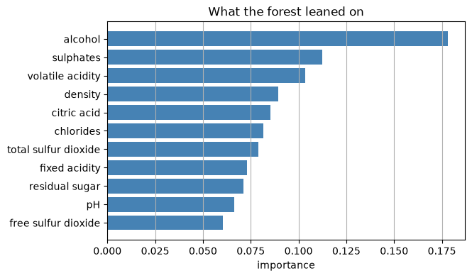
A forest keeps track of how much each feature helped, across all its questions in all its trees. sklearn calls this feature_importances_, and the numbers add up to 1.
# LEARN TO WRITE THIS. Which features did the forest use most?# Remember forest is the model that we trained above# do forest. (tab) will show you all of the things you can get from it# feature_importances_ is just one of those thingsimportance = pd.Series(forest.feature_importances_, index=X.columns) # one number per feature, they add to 1importance = importance.sort_values() # smallest first, so the biggest bar ends up on topprint(importance.sort_values(ascending=False).round(3))plt.figure(figsize=(6.5, 4))# Horizontal bar plotplt.barh(importance.index, importance.values, color="steelblue")plt.xlabel("importance")plt.title("What the forest leaned on")plt.grid(axis="x")plt.savefig("images/03-feature-importance.png", dpi=150, bbox_inches="tight")plt.show()
Alcohol is the forest’s favorite at 0.178, then sulphates and volatile acidity, the same three features our little two-question tree picked. That is reassuring.
Two warnings before you put a chart like this in a report.
Importance is not cause. It says what the forest found useful for predicting, not what makes a wine good. Pouring extra alcohol into a bottle will not make it a better wine.
Related features split the credit. Alcohol and density are correlated (the correlation is -0.496 on this data, because alcohol is lighter than water). When two features carry some of the same information, different trees use one or the other, and each one can look less important than the information really is.
Q7. Write this one out by hand
a. A winemaker reads the chart and says “so I should add more alcohol.” What would you tell them?
b. Suppose you added an exact copy of the alcohol column to the data, called alcohol2, and refit the forest. What would you expect to happen to the importance of alcohol? Why?
The Test Set, Once
Time to choose. Here is everything we tried, all scored on the same validation wines:
model
validation average precision
Day 5 logistic regression
0.532
one fully grown tree
0.299
bagging, 200 trees
0.641
random forest, 200 trees
0.667
The forest wins, so that is the model we take to the test set. We keep the Day 5 wine shop’s threshold of 0.3. Here is the forest at that threshold, still on validation.
# LEARN TO WRITE THIS. The forest at the shop's threshold, on validation.from sklearn.metrics import precision_score, recall_score, confusion_matrixy_pred_forest = (y_prob_forest >=0.3).astype(int)print("validation precision:", round(precision_score(y_valid, y_pred_forest), 3))print("validation recall: ", round(recall_score(y_valid, y_pred_forest), 3))
Precision 0.547 and recall 0.707. Day 5’s logistic regression at the same threshold had 0.521 and 0.61, so the forest is better on both. That is not a trade off, that is just a better model.
Every choice is made. Now, once:
# LEARN TO WRITE THIS. Score the test set once. Same forest, same threshold.y_prob_test = forest.predict_proba(X_test)[:, 1] # no scaler to worry about, trees do not need oney_pred_test = (y_prob_test >=0.3).astype(int)print(confusion_matrix(y_test, y_pred_test))print("test precision: ", round(precision_score(y_test, y_pred_test), 3))print("test recall: ", round(recall_score(y_test, y_pred_test), 3))print("test average precision:", round(average_precision_score(y_test, y_prob_test), 3))
[[321  25]
 [ 13  41]]
test precision:         0.621
test recall:            0.759
test average precision: 0.761
On 400 wines it never saw: precision 0.621, recall 0.759, average precision 0.761. Day 5’s logistic regression on the same test set, at the same threshold, got 0.54, 0.63, and 0.569. The forest finds 41 of the 54 good wines, and 41 of the 66 wines it flags really are good.
The test numbers came out higher than validation (0.761 against 0.667). Same as on Day 5, that is two different samples of wine wobbling, and it could have gone the other way. What matters is that the test set had no say in picking the forest or the threshold.
Q8. Write this one out by hand
a. Write the one sentence you would put in the report for the wine shop. Include the threshold, where it was chosen, and both precision and recall on the test set.
b. Why did we not also score logistic regression, bagging, and the single tree on the test set, and then report whichever did best?
Putting It Together
A decision tree asks yes or no questions, one feature at a time, and needs no scaling. Grown all the way it memorizes the training data: low bias, high variance.
A crowd of models only beats one model when their mistakes are different. Models trained on the same data mostly are not.
Bagging makes the trees different by giving each one its own bootstrap sample, then averages them. It fixes variance, not bias.
A random forest also hands each question a random handful of features, which makes the trees even more different. On wine it beat Day 5’s model on every number we care about.
Out-of-bag scores are free honest estimates from the wines each tree never saw.
Feature importance says what the forest used, not what causes what.
The rules from Days 4 and 5 do not change: choose on validation, open the test set once.
New Commands Today
Command
What it does
The thing that trips people up
DecisionTreeClassifier(max_depth=3)
a single tree
with no max_depth it grows until every leaf is pure, and overfits
no scaler needed, and training accuracy of 1.0 is normal here
oob_score=True, then .oob_score_
out-of-bag accuracy
it is accuracy, so compare it to the baseline. .oob_decision_function_[:, 1] gives the probabilities
.feature_importances_
how much each feature was used
they add to 1. Not cause, and related features split the credit
You Try: optional code
Nothing here is collected. Work through it if you want the idea to stick.
1. Refit tree_big with max_depth set to 3, 5, and 8. Which gives the best validation average precision? How close does the best single tree get to the forest?
2. In the forest, set max_features=None. Now every question can look at every feature, which makes it plain bagging. Does the validation average precision drop toward bagging’s 0.641?
3. Try min_samples_leaf=5 in the forest, which stops any leaf from holding fewer than 5 wines. Does it help or hurt here?
4. Use prompt 2 from the AI box in the Day 5 notes on max_features="sqrt": ask why the square root is the default for classification, and ask for a tiny example.
Before Next Class
In your lecture notes notebook, add your hand written notes and answers to the questions.
Do the Day 6 practice problems in HW_day6.ipynb.
Weekly Homework 3 is due Sunday 9/20 at 11:59pm. It covers Day 5 and Day 6, on real bank marketing data.
Read Geron chapter 6, the sections on Boosting and Stacking.
Watch the Day 7 video on the class website.
Day 7 is the other big way to build a crowd. Bagging trains its trees side by side and lets them vote. Boosting trains them one after another, and each new tree focuses on the wines the earlier ones got wrong.
Answers to the Q Boxes
Try every one of these by hand first. These are short summaries, not full answers, and the writing out is the part that does the work.
Q1. Reading the tree
a. Alcohol 12.1 is not at or below 11.15, so it goes right. Sulphates 0.80 is not at or below 0.705, so it goes right again. It lands in the far right leaf, value = [39, 52]. The tree predicts good, with probability 52 / 91 = 0.571.
b. Alcohol 9.8 is at or below 11.15, so it goes left. Volatile acidity 0.60 is above 0.325, so it goes right, into the leaf with 605 wines, value = [581, 24]. It predicts not good, with probability of good 24 / 605 = 0.04. The sulphates question only lives on the right branch, so a wine on the left branch never gets asked.
c. A tree only ever asks whether one feature is above a cutoff. Changing the units of a feature moves the cutoff but gives every wine the same answer. Logistic regression adds up weighted features, so a feature measured in big numbers can swamp the others unless you scale.
Q2. The big tree
a. Perfect training accuracy on noisy data means the model memorized the noise. It is the degree 15 polynomial from Day 2, and in Day 3’s words it is high variance. The validation score of 0.299 confirms it.
b. Any two of max_depth, min_samples_leaf, min_samples_split, and max_leaf_nodes. Each one stops the tree before every leaf is pure.
c. You would pick the one with the best validation score. But the scores differ mostly because of which wines each tree happened to get, so the best one is partly the luckiest one, and its validation score is optimistic. That is Day 4 again: the more things you try, the more the winner’s score includes luck.
Q3. Crowds
a. Each voter is right slightly more than half the time, and their mistakes are independent, so with many voters the wrong votes are spread out and the right answer almost always has more than half. Independence is the assumption that makes it work.
Q4. Bagging
a. A bootstrap sample draws rows from the training set with replacement until it has as many rows as the original. With replacement is what makes each sample different: some rows show up more than once and about a third never show up. Without it, every sample would just be the whole training set again.
b. From averaging. Each tree overfits to different noise because it saw a different sample. The real pattern shows up in most of the trees and survives the average, while the noise points in different directions and mostly cancels.
c. Variance. Bagging would not help a model whose problem is bias. Averaging many copies of a model that is too simple gives you an average that is still too simple.
Q5. Forests
a. At every question, each tree in a forest may only choose from a random handful of the features. That keeps a strong feature like alcohol from being the first question in every tree, so the trees are more different from each other and their mistakes cancel better.
b. Each tree is overfit to its own bootstrap sample, so each one is right on every training wine. But their mistakes on new wine are different, so the average of their probabilities is much better than any single tree.
c. Extra trees never make the forest worse, the curve is noisy, and 200 trees still trains in well under a second on this data. The cost is time and memory, which matters on big data.
Q6. Out-of-bag
a. Each wine is scored only by trees that never saw it during training, so the score is on data those trees did not fit, exactly like a validation set.
b. It is accuracy, and 86.4 percent of the wines are not good, so a model that never says yes gets 0.864. You need the baseline next to it, or a score made for rare positives like average precision.
c. If you use the out-of-bag score to make choices (how many trees, which settings), it becomes a validation score and picks up the same optimism. It also only works for bagged models, so it cannot referee a comparison against logistic regression. The test set is the one thing that never had a vote.
Q7. Importance
a. The forest found alcohol useful for telling good wines from not good ones in this data. That is a pattern, not a recipe. Good winemaking probably produces higher alcohol as a side effect, and adding alcohol to a finished wine does not change the things that made the good ones good.
b. It drops, and alcohol2 gets about the same amount. We tried it: alcohol went from 0.178 to 0.117 and alcohol2 got 0.12. Each question that wants alcohol uses whichever copy is in its random handful of features, so the credit is shared. Notice the two copies together (0.237) are worth more than alcohol was alone, because with two copies, alcohol shows up in more of the random handfuls. Either way the chart now shows two middling features where there is really one strong one, which is exactly the “related features split the credit” warning.
Q8. The test set
a. Something like: “At a threshold of 0.3, chosen on validation data, the random forest flags wines that are good 62 percent of the time and finds 76 percent of all good wines, measured on 400 wines it never saw.”
b. Because then the test set would be choosing the model. Whichever scored best would partly be the luckiest on those 400 wines, and the number you report would be optimistic. Choosing happens on validation, and the test set only scores the one model you already chose.