Blue Q boxes are questions for you to answer by hand, in a notebook, with a pen. Not because I am old fashioned. Writing something down by hand is slow, and slow is the point: it is very hard to write an explanation you do not actually understand. You are welcome to use AI in this class for the mechanics of code, but these boxes are the part where you do the thinking yourself. Bring your written notes to class, I will ask to see them.
Green You Try boxes are optional code for you to work through. Nothing is collected and nothing is graded. They are there because you will learn more from changing a number and rerunning than from watching me do it.
Every code cell begins with a tag that tells you what to do with it.
# RUN THIS. Setup, loading data, a plot. Copy it, run it, move on. You do not need to be able to write it from memory.
# LEARN TO WRITE THIS. The pattern of the day. The homework will ask you for it, and so will the exam. Type it out yourself at least once rather than pasting it.
# DEMO ONLY. Fake data or a contrived experiment that exists to show one idea. You would never write this for a real project and you do not need to be able to.
Short answers to the Q boxes are in drop down boxes at the very bottom. Write yours first.
Reading: Geron chapter 6, the sections on Boosting (both AdaBoost and Gradient Boosting) and Stacking.
Day 6 built a crowd by training a lot of trees at the same time and letting them vote. Every tree saw its own bootstrap sample, nobody was in charge, and the average cancelled out their mistakes.
Today we build a crowd the other way: one model at a time, each one fixing what the last one got wrong. That is boosting, and it is the other half of Geron chapter 6. It is a very popular way to build a classification model, one that can often be seen winning ML competitions.
It comes with a catch: with boosting, more trees can make the model worse, so we will have to be careful in choosing the number of trees.
Same wine data and the same test-train-validate splits as Day 5 and Day 6. One change: the test set stays closed today. We opened it on Day 6 to report the forest, and it does not get opened again just because we have a new model. Everything today happens on validation and on cross validation.
Setup
# RUN THIS. The same wine and the same splits as Day 5 and Day 6.import numpy as npimport pandas as pdimport matplotlib.pyplot as pltfrom sklearn.model_selection import train_test_splitwine = pd.read_csv("data/winequality-red.csv", sep=";")wine["good"] = (wine["quality"] >=7).astype(int)X = wine.drop(columns=["quality", "good"])y = wine["good"]X_train_full, X_test, y_train_full, y_test = train_test_split( X, y, test_size=0.25, stratify=y, random_state=42)X_train, X_valid, y_train, y_valid = train_test_split( X_train_full, y_train_full, test_size=0.25, stratify=y_train_full, random_state=42)print("training rows: ", X_train.shape[0])print("validation rows:", X_valid.shape[0])print("test rows: ", X_test.shape[0])
training rows:   899
validation rows: 300
test rows:       400
What Boosting Does
The core idea: instead of building one big model that tries to get everything right at once, or build lots of full models and let them vote, we build many small models in sequence, where each one’s only job is to fix the mistakes of everyone before it.
The steps
Start with one small tree. It gets a lot wrong. It’s a bad model on its own, and that’s fine.
Compute the residual: actual value minus current prediction. This is the part of the answer the model hasn’t explained yet.
Train a new small tree whose target is predicting the residual, not the original y-values. Then add a fraction of that new tree’s output to the running total (the fraction is called the learning rate and it just keeps any single tree from overcorrecting).
Repeat, hundreds of times. Each tree only ever sees what’s currently wrong, so it only ever tries to fix that.
Nobody votes, and nothing is averaged. The models are added together, running total plus one small correction, plus another small correction, and so on.
Why “residual” is really “gradient” - remember the derivative!
To minimize a function numerically we take the derivative (find the slope at a point), and step against it, try to walk downhill.
Gradient boosting does the same thing, except the thing being optimized isn’t a single number x, it’s the model’s entire vector of predictions (\hat y_1, \hat y_2, \dots, \hat y_n), one per data point. The function being minimized is total squared error:
L = \sum_i (y_i - \hat y_i)^2
Where L is the loss function. Take the derivative of L with respect to a single prediction \hat y_i (everything else held fixed, just applied one coordinate at a time):
The thing in parentheses is the residual (error), up to a constant factor. So “to train a tree on the leftovers” is “take a step in the direction that decreases total error,” in exactly the sense you learned in calculus or math for data science, just with one derivative per data point instead of one derivative total.
F_{\text{new}}(x) = F_{\text{old}}(x) + \eta \cdot (\text{tree fit to residuals})
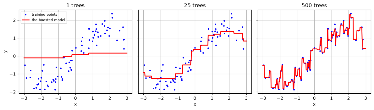
The effect is easiest to see on a simple made up data set, so we can plot the model itself. Below, the blue dots are training points and the red line is the boosted model after 1 tree, after 25 trees, and after 500 trees.
# DEMO ONLY. A fake curve with noise, so we can watch boosting build a model.from sklearn.ensemble import GradientBoostingRegressorrng = np.random.default_rng(42)x = np.sort(rng.uniform(-3, 3, 120)) # 120 points between -3 and 3y_fake = np.sin(x) +0.3* x + rng.normal(0, 0.35, 120) # a curve, plus noiseX_fake = x.reshape(-1, 1) # sklearn wants a column, not a rowX_fake_train, X_fake_valid, y_fake_train, y_fake_valid = train_test_split( X_fake, y_fake, test_size=0.35, random_state=0)# Choose x-values just for plottinggrid = np.linspace(-3, 3, 400).reshape(-1, 1) # Make three subplotsfig, axes = plt.subplots(1, 3, figsize=(12, 3.6), sharey=True)# NEW COMMAND? zip makes an iterable that contains tuples that can be unpacked in a for loop.for ax, n inzip(axes, [1, 25, 500]): model = GradientBoostingRegressor( n_estimators=n, # how many trees to add, one after another learning_rate=0.1, # how much of each new tree to add. More on this below max_depth=2, # each tree is tiny on purpose random_state=42) model.fit(X_fake_train, y_fake_train) ax.plot(X_fake_train, y_fake_train, "b.", markersize=5, label="training points") ax.plot(grid, model.predict(grid), "r-", linewidth=2, label="the boosted model") ax.set_title(str(n) +" trees") ax.grid() ax.set_xlabel("x")axes[0].set_ylabel("y")axes[0].legend(fontsize=8)plt.tight_layout()plt.savefig("images/01-boosting-stages.png", dpi=150, bbox_inches="tight")plt.show()
Here the red line is our Gradient Boost Regressor model. It has jumps in its answer as it crosses decision boundaries that the tree finds.
With 1 tree the model is a couple of flat steps. It is a tree of depth 2, so that is all it can be. With 25 trees it has found the shape of the curve. With 500 trees it is chasing individual points, including the noise.
That last panel should make you think…. HIGH VARIANCE. This is different from the random forest when adding more trees was always better. Here 500 trees seems to be overfitting!
Q1. Write this one out by hand
a. In your own words, what does each new tree in a boosted model get trained on? How is that different from each new tree in a random forest?
b. In the 500 tree panel, the red line passes very close to nearly every blue dot. Why is that bad, given how y_fake was built?
c. Bagging trains its trees at the same time and boosting trains them one after another. Which one can you speed up by using more cores of your computer? Why?
More Trees Can Make It Worse
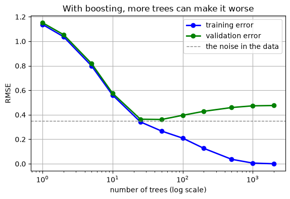
On Day 6 we added trees to the forest and the score went up and then flattened out. Extra trees cost time and nothing else. Boosting is not like that. Each new tree is fitted to what is left over, so once the real pattern is used up, the new trees start fitting the noise.
Let’s plot a learning curve!
Q2. Write this one out by hand
a. What is a learning curve?
# DEMO ONLY. Training and validation error as we add trees to a boosted model.from sklearn.metrics import mean_squared_errortree_counts = [1, 2, 5, 10, 25, 50, 100, 200, 500, 1000, 2000]train_errors = []valid_errors = []for n in tree_counts: model = GradientBoostingRegressor(n_estimators=n, learning_rate=0.1, max_depth=2, random_state=42) model.fit(X_fake_train, y_fake_train) train_rmse = mean_squared_error(y_fake_train, model.predict(X_fake_train)) **0.5 valid_rmse = mean_squared_error(y_fake_valid, model.predict(X_fake_valid)) **0.5 train_errors.append(train_rmse) valid_errors.append(valid_rmse)print("trees", n, " training RMSE", round(train_rmse, 3), " validation RMSE", round(valid_rmse, 3))plt.figure(figsize=(6.5, 4))plt.semilogx(tree_counts, train_errors, "b-o", linewidth=2, label="training error")plt.semilogx(tree_counts, valid_errors, "g-o", linewidth=2, label="validation error")plt.axhline(0.35, color="gray", linestyle="--", linewidth=1, label="the noise in the data")plt.xlabel("number of trees (log scale)")plt.ylabel("RMSE")plt.title("With boosting, more trees can make it worse")plt.grid()plt.legend()plt.savefig("images/02-too-many-trees.png", dpi=150, bbox_inches="tight")plt.show()
trees 1   training RMSE 1.138   validation RMSE 1.152
trees 2   training RMSE 1.038   validation RMSE 1.054
trees 5   training RMSE 0.8   validation RMSE 0.819
trees 10   training RMSE 0.561   validation RMSE 0.576
trees 25   training RMSE 0.342   validation RMSE 0.364
trees 50   training RMSE 0.267   validation RMSE 0.362
trees 100   training RMSE 0.21   validation RMSE 0.396
trees 200   training RMSE 0.126   validation RMSE 0.428
trees 500   training RMSE 0.037   validation RMSE 0.459
trees 1000   training RMSE 0.006   validation RMSE 0.473
trees 2000   training RMSE 0.0   validation RMSE 0.476
Validation error, the green line, falls to 0.362 at 50 trees, which is about as good as it can get, because the noise we added has a standard deviation of 0.35. Then it climbs back up: 0.396 at 100 trees, 0.459 at 500, and 0.476 at 2000. Meanwhile the blue line marches to 0.000. At 2000 trees the model reproduces every training point exactly and is worse than useless on new points. The big gap between the training and validation error is a clear indicator of overtraining.
So n_estimators in boosting is not “bigger is safer” like it was for a forest. It is a real parameter you have to think about, and the way you set it is by using the validation set.
Q3. Write this one out by hand
a. On Day 6 we said more trees never hurt a random forest. Explain why boosting is different, in terms of what each new tree is trained on.
b. The validation error bottoms out at 0.362 and the noise in the data has a standard deviation of 0.35. Why can no model, however clever, get the validation error much below 0.35 here?
c. Suppose you only looked at the training error in that table. What would you conclude about 2000 trees, and what would go wrong when you used the model?
The Learning Rate
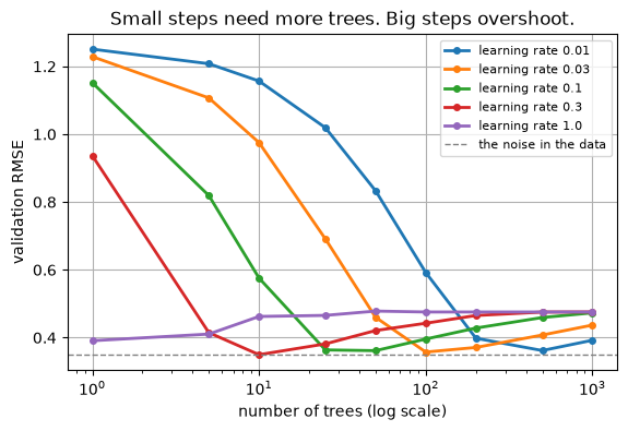
There is a second parameter in our model, and it works against the first one. learning_rate says how much of each new tree to add. AKA how big of a step to take in the direction of the negative of the derivative. A small learning rate means every tree is a small correction, so you need many of them (lots of steps). A big one means each tree changes the model a lot (but you could take a big step in a bad direction).
NOTE: Notice again here that we are using a for loop to explore the effect of parameters on our model. While this would not belong in your results, it’s a good idea to have in your back pocket!!!
# DEMO ONLY. The same fake curve, different learning rates.learning_rates = [0.01, 0.03, 0.1, 0.3, 1.0]counts = [1, 5, 10, 25, 50, 100, 200, 500, 1000]plt.figure(figsize=(6.5, 4))for rate in learning_rates: errors = []for n in counts: model = GradientBoostingRegressor(n_estimators=n, learning_rate=rate, max_depth=2, random_state=42) model.fit(X_fake_train, y_fake_train) errors.append(mean_squared_error(y_fake_valid, model.predict(X_fake_valid)) **0.5) best =min(errors) best_n = counts[errors.index(best)]print("learning rate", rate, " best at", best_n, "trees, validation RMSE", round(best, 3)) plt.semilogx(counts, errors, "-o", linewidth=2, markersize=4, label="learning rate "+str(rate))plt.axhline(0.35, color="gray", linestyle="--", linewidth=1, label="the noise in the data")plt.xlabel("number of trees (log scale)")plt.ylabel("validation RMSE")plt.title("Small steps need more trees. Big steps overshoot.")plt.grid()plt.legend(fontsize=8)plt.savefig("images/03-learning-rate.png", dpi=150, bbox_inches="tight")plt.show()
learning rate 0.01   best at 500 trees, validation RMSE 0.362
learning rate 0.03   best at 100 trees, validation RMSE 0.358
learning rate 0.1   best at 50 trees, validation RMSE 0.362
learning rate 0.3   best at 10 trees, validation RMSE 0.35
learning rate 1.0   best at 1 trees, validation RMSE 0.391
Here we are increasing the number of trees on the x-axis, and tracking 5 different learning rate choices. We know the noise in the data based on the standard deviation we chose in our randomness when we generated the data.
Look at where each curve bottoms out.
learning rate
best number of trees
best validation RMSE
0.01
500
0.362
0.03
100
0.358
0.1
50
0.362
0.3
10
0.350
1.0
1
0.391
The first four all reach about the same error, they just need different numbers of trees to get there. Small learning rate, many trees. Big learning rate, few trees. At 1.0 the model takes steps so large that it never settles, and the best it manages is a single tree. So how do we know what is best?
learning_rate and n_estimators are one decision, not two. Lower one and you must raise the other. Be careful not to use large learning rates, big steps struggle to converge to a good answer.
A small learning rate seems like a good choice, but with too many trees starts to overfit. Ideally you stop adding trees before you overfit! Doing this automatically is called early stopping, and it is the next section.
Q4. Write this one out by hand
a. Your model uses learning_rate=0.1 with 50 trees. You want to try learning_rate=0.01. Roughly what should you do to n_estimators, and why?
b. Why does a learning rate of 1.0 do worse than every smaller rate here, even with 1000 trees available?
c. A friend says “I will just set learning_rate very small and n_estimators very large, that must be safest.” What does the plot say happens, and what does it cost?
Boosting on the Wine
Let’s try this on our Wine data! Here is gradient boosting as a classifier, on the wine, scored the Day 5 way on the same validation wines.
NOTE: We can do decision trees as either a regressor or classifier!! Keep in your mind what task you are doing! Above we did regression and discussed results in terms of RMSE. With the wine classification data we need to use accuracy, precision, recall, etc.
# LEARN TO WRITE THIS. Gradient boosting on the wine.from sklearn.ensemble import GradientBoostingClassifierfrom sklearn.metrics import average_precision_scoreboosted = GradientBoostingClassifier( n_estimators=200, max_depth=5, # Start deeper than above learning_rate=0.1, # A good starting place random_state=42)boosted.fit(X_train, y_train)y_prob_boost = boosted.predict_proba(X_valid)[:, 1]print("gradient boosting, validation average precision:", round(average_precision_score(y_valid, y_prob_boost), 3))
gradient boosting, validation average precision: 0.673
Okay, so using boosting with 200 trees and a max depth of 5 we got 0.673 average precision. Compare that to Day 6’s random forest, which got 0.667 on these same wines. So we made some progress. We can discuss later how much progress we actually made.
XGBoost
XGBoost is another gradient boosting method. It is a separate package, not part of sklearn, and it is the tool people reach for. It does the same thing as gradient boost, but it is optimized for computational speed and adds in the ability to regularize.
The good news for you: it copies sklearn’s interface, so fit, predict and predict_proba all work exactly as you expect.
# LEARN TO WRITE THIS. XGBoost, which behaves like an sklearn model.import xgboost as xgbxgb_model = xgb.XGBClassifier( n_estimators=200, learning_rate=0.1, max_depth=3, random_state=42, eval_metric="logloss") # what it watches while training. # logloss is the usual default for classificationxgb_model.fit(X_train, y_train)print("XGBoost, validation average precision:",round(average_precision_score(y_valid, xgb_model.predict_proba(X_valid)[:, 1]), 3))
XGBoost, validation average precision: 0.605
We get an average precision of 0.605 with 200 trees, and it fits in a fraction of a second.
The other thing about XGBoost is that it can watch a validation set while it trains and stop by itself! When the validation score stops improving the model stops adding trees.
Early Stopping
Early stopping is a machine learning method that helps control for overfitting. It is useful in any model where you train using iterative steps. Here we iterate by building successive models each of which get us closer to a best score. Iterative models have a bad habit of overfitting if they are left to train too long. So we keep track of how the model is doing on the training and validation sets as we are training and stop training once the results on our validation set start to get worse after many rounds (validation error is not a smoothly decreasing thing).
# LEARN TO WRITE THIS. Let XGBoost decide how many trees to use.xgb_early = xgb.XGBClassifier( n_estimators=2000, # an upper limit, not a promise. It will stop long before this learning_rate=0.05, max_depth=3, random_state=42, eval_metric="aucpr", # watch the precision/recall area, the Day 5 score for rare positives early_stopping_rounds=50) # stop when 50 trees in a row fail to improve itxgb_early.fit( X_train, y_train, eval_set=[(X_valid, y_valid)], # the set it watches. Never the test set verbose=False)print("it stopped at tree:", xgb_early.best_iteration, "out of 2000")print("validation average precision:",round(average_precision_score(y_valid, xgb_early.predict_proba(X_valid)[:, 1]), 3))
it stopped at tree: 193 out of 2000
validation average precision: 0.622
XGBoost stopped at tree 193 and scored 0.622. We never had to guess n_estimators: we gave it a ceiling of 2000 and it found its own stopping point.
One thing to be clear about. The validation set is being used to make a choice here, which is exactly what a validation set is for. The test set is not involved, and the number you report at the end still has to come from data that had no say in any choice when you were building the model.
Q5. Write this one out by hand
a. What does early_stopping_rounds=50 actually mean? Why not stop the first time a tree fails to improve the score?
b. Why is it fine to early stop on the validation set, but not on the test set?
c. We gave n_estimators=2000 and it used 193. Would setting n_estimators=300 have changed the answer here? What about n_estimators=100?
Is the Boosted Model Actually Better?
Gradient boosting got 0.673 average precision on validation and the random forest from last lecture got 0.667. That is a win of 0.006… right?
BEWARE! It is important to keep in mind your data. The validation set contains only 41 good wines out of 300, or about 13.6 percent, and if just one of those wines moved from good to bad it would be 13.3 percent. A single bottle being reclassified moves our data more than that 0.006 that we claim is a win.
So compare them properly. We will use a cross_val_score with repeated stratified folds. This fits each model many times on different splits of the training data, and gives us a spread instead of one number, so we can really say how important that 0.006 was.
In previous classes we talked about StratifiedKFold(). Adding Repeated to this just lets the model repeat the sampling of the folds multiple times so that we don’t get some advantage from how we picked our folds.
# LEARN TO WRITE THIS. Compare two models with repeated cross validation.from sklearn.model_selection import cross_val_score, RepeatedStratifiedKFoldfrom sklearn.ensemble import RandomForestClassifier# Cross Validationcv = RepeatedStratifiedKFold( n_splits=5, # 5 folds n_repeats=4, # done 4 times with different shuffles, so 20 fits per model random_state=42)# Compare two modelsforest = RandomForestClassifier(n_estimators=200, random_state=42)boost = GradientBoostingClassifier(n_estimators=200, max_depth=5, random_state=42)for name, model in [("random forest", forest), ("gradient boosting", boost)]: scores = cross_val_score(model, X_train_full, y_train_full, cv=cv, scoring="average_precision")print(name)print(" mean average precision:", round(scores.mean(), 3))print(" standard deviation: ", round(scores.std(), 3))print(" worst and best fold: ", round(scores.min(), 3), "to", round(scores.max(), 3))
random forest
   mean average precision: 0.633
   standard deviation:     0.084
   worst and best fold:    0.442 to 0.764
gradient boosting
   mean average precision: 0.611
   standard deviation:     0.086
   worst and best fold:    0.449 to 0.774
The random forest averages 0.633 and the boosted model 0.611, and both wobble by about 0.085 from fold to fold. The gap between the two models is a quarter of the noise in the measurement, and it points the other way from the single validation number.
The honest conclusion: on this data, with these settings, the two models are tied. Boosting did not beat the forest. A 0.006 lead on one validation set was never evidence of anything.
This is worth more than it looks. It is very easy to try six models, report the highest number, and believe it. The cure is cheap: compare with repeated cross validation, look at the spread, and only claim a winner when the gap is bigger than the wobble. This is truly a pro move when comparing how multiple different models did!!
And notice what we did not do: open the test set to break the tie. PRO MOVE!
Q6. Write this one out by hand
a. Why is a mean over 20 fits more trustworthy than one validation score, even though both use data the model did not train on?
b. The standard deviation was about 0.085. Explain, to somebody who has not taken this class, why a difference of 0.006 between two models does not mean much next to that.
c. We have two tied models. Give one reason you might ship the forest and one reason you might ship the boosted model, neither of which is the score.
Where Boosting Does Win
Our wine set is small (1199×11). Boosting can still win here, but you need to be careful. Use shallow trees, low learning rate, and early stopping since there’s less data to average out overfitting. As datasets get bigger, that need for babysitting drops and boosting’s natural advantages kick in, so XGBoost is my default once data gets large, unless I’ve got a specific reason to reach for something else.
Stacking, in One Paragraph
The last section of Geron chapter 6 is stacking. Instead of averaging or adding models, you train a final model whose input is the other models’ predictions. It learns how much to trust each one. The catch: you can’t train it on predictions the base models made on their own training data, since that’s already overfit. You need out-of-fold predictions to train this final model. This is a useful method for edging out a win in an ML competition, but not my go to method. You spend a lot of extra time and data for only a fraction of return.
Q7. Write this one out by hand
a. In your own words, what does the final estimator in a stack take as its input?
b. Stacking scored 0.668, the forest 0.667, boosting 0.673. Using what you learned in the repeated cross validation section, what should you say about these three numbers?
Putting It Together
bagging and forests (Day 6)
boosting (today)
how the trees are built
all at once, independently
one after another, each fixing the last
what each tree sees
its own bootstrap sample
what the model still gets wrong
more trees
never hurts, just slower
can overfit, so it is a real choice
main parameters
n_estimators, max_features
learning_rate with n_estimators, max_depth
how to set the number of trees
as many as you can afford
early stopping on a validation set
runs in parallel
yes
not really, each tree needs the one before
typical use
a strong, safe default
usually the best score on tables of numbers
The recipe for today’s family:
Start with learning_rate=0.05 or 0.1 and a small max_depth (3 is a good first try).
Set n_estimators high and let early stopping pick the real number, watching a validation set.
Compare against a random forest with repeated cross validation, not one split.
Only claim a winner when the gap is bigger than the fold-to-fold wobble.
The test set stays closed until everything is decided.
slow, and rarely worth it. cv=5 keeps the members’ predictions honest
You Try: optional code
Nothing here is collected. Work through it if you want the idea to stick.
1. In the wine gradient boosting cell, try max_depth=2 and max_depth=8. Which does better on validation? Boosting usually likes shallow trees, does the wine agree?
2. Give the XGBoost early stopping cell learning_rate=0.01 instead of 0.05. Where does it stop now, and does the score change? This is the trade off from the learning rate section, on real data.
3. Run the repeated cross validation comparison again with n_repeats=10. Does the gap between the forest and the boosted model look any more real with 50 fits?
4. Build a StackingClassifier with the forest, the boosted model, and logistic regression, and see whether it beats either one on its own. It takes a few seconds to fit. Was it worth the wait?
Before Next Class
In your lecture notes notebook, add your hand written notes and answers to the questions.
Do the Day 7 practice problems in HW_day7.ipynb.
Weekly Homework 4 is due Sunday 9/27 at 11:59pm. It covers Day 7 and Day 8.
Read Geron chapter 2, all of it. It is the end to end project chapter, and Day 8 follows it.
Watch the Day 8 video on the class website.
Day 8 puts the whole thing together: one pipeline that takes raw data in one end and a tuned, evaluated model out the other. Everything since Day 2 has been a piece of that pipeline.
Answers to the Q Boxes
Try every one of these by hand first. These are short summaries, not full answers, and the writing out is the part that does the work.
Q1. What boosting does
a. Each new tree is trained on what the model so far still gets wrong, the leftovers or residuals. In a random forest every tree is trained on its own bootstrap sample of the original data and never looks at the other trees.
b.y_fake is a smooth curve plus random noise. A line that passes through nearly every point has fitted the noise, which is different for every new sample, so it will do worse on new points. That is the 500 tree panel.
c. Bagging. Its trees do not depend on each other, so a computer with eight cores can build eight at a time (that is what n_jobs does). Boosting cannot start a tree until the one before it is finished.
Q2. Learning curves
a. A learning curve is a plot of how the model does as you give it more of something, with the training score and the validation score on the same axes. On Day 2 the x axis was how many training rows the model got. Today it is how many trees we have added. You read the shape: while both curves fall together the model is still learning, and when the validation curve turns back up while the training curve keeps falling, the model has started memorizing. The bottom of the validation curve is where you want to stop.
Q3. Too many trees
a. A forest averages independent trees, so extra trees only make the average steadier. A boosted model keeps adding corrections to itself, and once the real pattern is used up the only thing left to correct is noise, so the extra trees fit noise.
b. The data itself carries noise with a standard deviation of 0.35. Even a model that knew the true curve exactly would miss each point by about that much. No model can predict a coin flip.
c. The training error at 2000 trees is 0.000, so you would conclude it is a perfect model. On new data it is the worst model in the table, 0.476 against 0.362 for 50 trees.
Q4. Learning rate
a. Raise n_estimators, by roughly the same factor you lowered the rate. In the table, 0.1 needed 50 trees and 0.01 needed 500.
b. Each tree is added at full strength, so the model overshoots the answer, and later trees spend their time undoing those overshoots. Its best score came from a single tree.
c. A tiny learning rate with a huge number of trees still overfits, the curve just takes longer to turn upward, and every one of those trees costs time. What you want instead is to stop at the bottom of the curve.
Q5. Early stopping
a. It keeps going until 50 trees in a row have failed to improve the validation score, then stops and keeps the best one. Stopping at the first failure would quit far too early, because the score wobbles up and down from tree to tree even while it is still improving overall.
b. Stopping early is a choice, the choice of how many trees. Choices are made on validation data. If the test set made that choice, its score would include that choice and would no longer be an honest estimate.
c.n_estimators=300 would give the same model, since it stopped at 193 on its own. n_estimators=100 would cut it off before it was done, and you would never know, because it would simply run out of trees rather than stop.
Q6. Tied models
a. One validation score is a single sample: these particular 300 wines, of which only 41 are good. The mean over 20 fits uses every training wine as held out data at some point, so it averages out which wines happened to land where.
b. Say the two models were measured with a ruler that wobbles by about 0.085 every time you use it. A difference of 0.006 is far smaller than the wobble, so you cannot tell the models apart with it. You would need either a much bigger gap or a much steadier ruler.
c. Reasons for the forest: it has fewer parameters to get wrong, it trains in parallel, and out-of-bag scoring is free. Reasons for boosting: it usually scales better to bigger data, early stopping picks the tree count for you, and XGBoost is what the industry expects to see. Either is defensible when the scores are tied.
Q7. Stacking
a. The predictions of the member models. Each member makes a prediction for a row, and those predictions become the features the final estimator learns from, which is how it learns whom to trust when.
b. They are tied. All three sit inside the fold-to-fold wobble we measured, so ranking them by the third decimal place is reading noise. Pick on training time, simplicity, or what your team can maintain.