Machine learning (ML) is a field of study in artificial intelligence concerned with the development and study of statistical algorithms that can learn from data and generalise to unseen data, and thus perform tasks without explicit instructions.
Broadly speaking it is a field that was built out of statistical modeling. Even though there has been a boom in machine learning in the past few years, it is a field that has actually been around since the early 1900.
Machine Learning and Data Science
In the data science lifecycle you often move toward modeling and prediction after your initial EDA (exploratory data analysis). You have looked at the data and noticed patterns and start to wonder “can I predict something using this data?”. In some cases you will use machine learning as part of this process.
Some examples include:
Linear or logistic regression
Time series and forecasting
Pattern recognition
Dimensionality reduction
Neural networks and Classifiers
ML Process
Acquire and clean the data
Exploratory data analysis
Test - Train - Validate data split
Data wrangling - feature engineering
Model Training
Hyperparameter Tuning
Model Testing
Model Deployment or Publication
Check your installs:
import sysprint("Python version:", sys.version)import pandas as pdprint("pandas version:", pd.__version__)import matplotlibprint("matplotlib version:", matplotlib.__version__)import numpy as npprint("NumPy version:", np.__version__)import scipy as spprint("SciPy version:", sp.__version__)import IPythonprint("IPython version:", IPython.__version__)import sklearnprint("scikit-learn version:", sklearn.__version__)
If you are missing any of these packages then please install them!
!conda install -y pacakge_name
# Some basic package importsimport osimport numpy as npimport pandas as pd# Visualization packagesimport matplotlib.pyplot as pltimport plotly.express as pxfrom plotly.subplots import make_subplotsimport plotly.io as pioimport seaborn as sns
Example ML project
We are going to explore a start to finish mini-machine learning project. This is like your “Hello World” introduction. As we move through the rest of the semester we will go into much more detail about model selection, training, etc.
Classification
One thing that machine learning models tend to be very good at is classification tasks. Classification is when a model takes input variables for an observation and figures out how to classify the observation from that data. For example, given a photo is it a cat or a dog?
The Data
The Iris dataset contains measurements of iris flowers from three different species. The dataset was first introduced by Sir Ronald A. Fisher in 1936. The measurements themselves were originally collected by Edgar Anderson, a botanist who studied the morphology of iris flowers from three related species.
Number of samples: 150 Number of features or variables: 4 (all numeric and continuous)
Features: - sepal length (in cm) - sepal width (in cm) - petal length (in cm) - petal width (in cm)
From looking at the value_counts() we see our data is well balanced. Balanced data is important in prediction. If we only had, say, three or four observations of the setosa species we likely would not be very accurate in predicting that class.
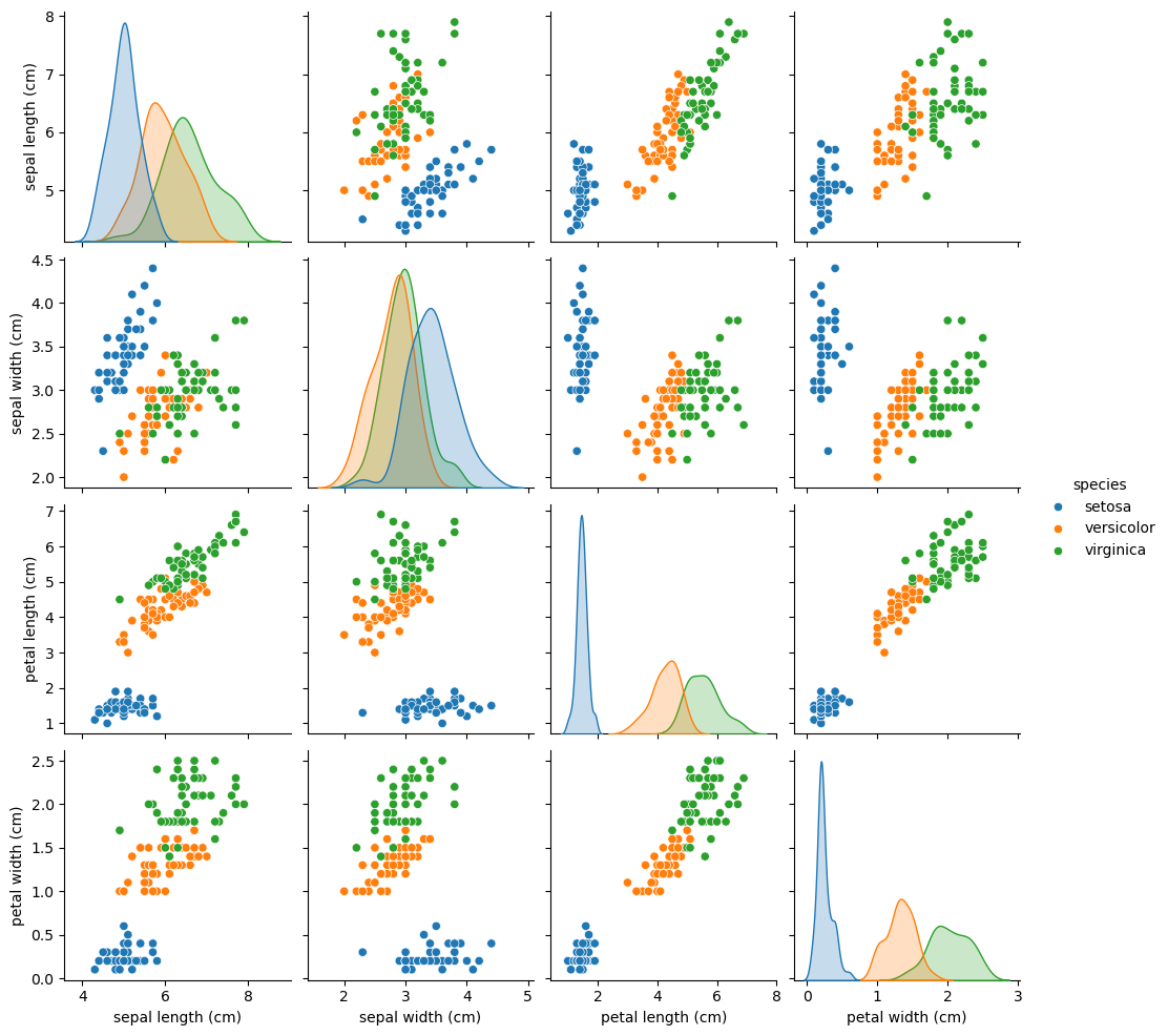
We also want to look at some visualizations. Does it seem reasonable that the variables we have could be used for classification? Are there strange outliers?
Here we will do a pairplot and color it by the thing we want to predict (‘species’)
sns.pairplot(df,hue='species')
Train - Test Split
Before we get too deep into the analysis, but after we are fairly certain that our data is clean and could be usefull for classification, we want to do a train test split.
WHY SPLIT?
If you trained a prediction model using all the data and then test it using the same data there is a real concern that the model will just memorize the data. It will get really great at predicting the data you have, but will be useless at predicting new, future, data. This is just like taking an exam!
If you had a teacher who gave you the whole exam (all the data) and then said, learn this. The best way to do that is to memorize the exam. Any you would get really good at taking that exam. But how good would you be at applying that knowledge to new scenarios? Probably not great!
Now instead imagine you have a teacher that gives you lots of practice problems (a training set) and then choose a new set of problems on the exam for you to apply your knowledge to (a test set). If you can pass the test, then it is fairly likely that you will be able to apply your knowledge to new scenarios and memorizing the training set would not help.
So we split our data into Testing, Training, and sometimes Validation sets:
Training - about 80% of the data that the model gets to see when learning. (homework) Validation - about 10% of the data that the scientists uses to tune the model (like a practice exam) Testing - about 10% of the data that is the real text to see how accurate your model actually was (a final exam)
You want to be the best teacher you can be!
The train_test_split function from sklearn.model_selection helps us separate our data randomly. Here is how it’s used:
You send in as many data sets as you want. Here we send in our features or (variables) the \(X\) data, and our target (predictions or species) the \(y\) data. In genera we want a function that tells us
\[ y = F(X) \]
where we send in \(X\) and get out \(y\). We can do optional arguments, here test_size = .2 says to use 20% of the data for testing, and setting a random_seed makes the results reproducible.
Data shape mismatch errors are very common and very frustrating. You may as well check to see that the data shapes are what you expect.
First we see that the \(X\) data has 4 columns and this matches our four input variables. We see that training has 120 observations and testing has 30. This means 20% of the data really did end up in testing and 80% in training. If we look at the \(y\) data it has one column - just the species we want to predict.
Often you have to reshape because the ML algorithms expect the data in a certain format. In our case we want our training data to be interpreted as a list of predictions, no extra columns. So we reshape it:
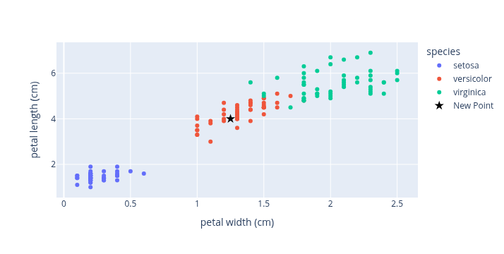
At this point we could choose a wide range of possible models. We will do a very simple model called K-Nearest Neighbors (KNN). KNN is one of the simplest ways for a computer to make predictions based on data. When the computer sees a new example, it looks at the K most similar examples it has already seen - its “nearest neighbors”. If most of those neighbors belong to a certain group, the computer guesses that the new example belongs to that group too. For instance, if most nearby flowers are iris setosa, it will predict the new flower is also setosa.
If we look at the nearest neighbors around the new point we see that it is very likely a member of Versicolor. We can choose how many neighbors to consider. I often start with just 1 or 2. The distance to the nearest neighbor can be calculated quite a few ways:
Distance Metric
Formula / Idea
When to Use
Euclidean distance
Straight-line distance between two points. ( d = )
Default for continuous, numeric data. Works well when all features are on the same scale.
Manhattan distance (L1 norm)
Distance along grid lines (like city blocks). ( d =
x_i - y_i
)
Useful when features are independent or you want to reduce the effect of outliers.
Minkowski distance
General form that includes Euclidean and Manhattan as special cases. ( d = (
x_i - y_i
p){1/p} )
Choose (p=1) → Manhattan, (p=2) → Euclidean.
Chebyshev distance
Maximum coordinate difference. ( d =
x_i - y_i
)
Good for problems where only the largest difference matters.
Cosine distance
Based on the angle between two vectors, not magnitude. ( d = 1 - )
Common for text or high-dimensional data (like word embeddings).
Hamming distance
Counts how many features differ.
Used for categorical or binary features.
Default is Minkowski and it is usually perfect for a first try.
Define the model in Python
from sklearn.neighbors import KNeighborsClassifierknn = KNeighborsClassifier(n_neighbors=1)
Train the Model
For KNN this is a simple as storing the training data and species types so that when it gets a new observation it has something to compare to.
knn.fit(X_train, y_train)
KNeighborsClassifier(n_neighbors=1)
In a Jupyter environment, please rerun this cell to show the HTML representation or trust the notebook. On GitHub, the HTML representation is unable to render, please try loading this page with nbviewer.org.
Parameters
n_neighbors
1
weights
'uniform'
algorithm
'auto'
leaf_size
30
p
2
metric
'minkowski'
metric_params
None
n_jobs
None
KNeighborsClassifier Parameters Explained
1. n_neighbors (default = 5)
- The K in KNN - the number of nearest neighbors the algorithm looks at when making a prediction.
- Example: n_neighbors=3 - it looks at the 3 closest points.
2. weights (default = ‘uniform’)
- Determines how neighbors are counted:
- 'uniform' - all neighbors are equally important.
- 'distance' - closer neighbors count more than farther ones.
3. algorithm (default = ‘auto’)
- Chooses the method to find nearest neighbors:
- 'auto' - automatically picks the best method.
- 'ball_tree', 'kd_tree', 'brute' - different search methods.
4. leaf_size (default = 30)
- Used with tree-based algorithms (kd_tree, ball_tree).
- Controls the size of leaf nodes in the tree (affects speed, not accuracy).
5. p (default = 2)
- The power parameter for the Minkowski distance:
- p = 1 - Manhattan distance
- p = 2 - Euclidean distance
6. metric (default = ‘minkowski’)
- The distance metric used to measure “closeness”:
- 'euclidean' - straight-line distance
- 'manhattan' - city-block distance
- 'minkowski' - general formula (p = 1 → Manhattan, p = 2 → Euclidean)
7. metric_params (default = None)
- Extra parameters for the distance metric. Usually leave as None.
8. n_jobs (default = None)
- How many CPU cores to use for computation:
- None - uses 1 core
- -1 - uses all available cores (faster for large datasets)
Simple summary
n_neighbors - how many friends to ask
weights - do all friends count equally?
algorithm & leaf_size → how to find friends efficiently
p & metric - how to measure closeness
n_jobs - how many cores to use
Try a Prediction
Now that the model is trained you can see what happens in a prediction. Here we will make up a data point (a pretend flower) and see what the models does with this information.
# Create some new dataX_new = pd.DataFrame([[5, 2.9, 1, 0.2]],columns=df.keys()[0:4])print("X_new.shape:", X_new.shape)
Great the model is giving at least reasonable outputs. It if had an error our give an answer of 72, or “dog” or something we would know we already had a problem.
Model Testing (or Validation)
Now we want to see how our model does on the exams. We are now giving it data that it did not see during the training phase to check if it can do a good job predicting that data. When we call
knn.predict()
we are sending \(X\) data into our model \(F(x)\) to see what it returns as the \(y\) value, in this case a category.
y_pred = knn.predict(X_test)print("Test set predictions:\n", y_pred)