# NOTE - This list of package imports is getting long
# In a professional setting you would only want to
#      import what you need!
# I had chatGPT break the packages into groups here

# ============================================================
# Basic packages
# ============================================================
import os                             # For file and directory operations
import numpy as np                    # For numerical computing and arrays
import pandas as pd                   # For data manipulation and analysis

# ============================================================
# Visualization packages
# ============================================================
import matplotlib.pyplot as plt        # Static 2D plotting
from matplotlib.colors import ListedColormap
import seaborn as sns                  # Statistical data visualization built on matplotlib

# Interactive visualization with Plotly
import plotly.express as px
from plotly.subplots import make_subplots
import plotly.io as pio
pio.renderers.default = 'colab'        # Set renderer for interactive output in Colab or notebooks

# ============================================================
# Scikit-learn: Core utilities for model building and evaluation
# ============================================================
from sklearn.model_selection import train_test_split    # Train/test data splitting
from sklearn.preprocessing import PolynomialFeatures, MinMaxScaler, StandardScaler  # Feature transformations and scaling
from sklearn.metrics import (                            # Model evaluation metrics
    mean_squared_error, r2_score, accuracy_score,
    precision_score, recall_score, confusion_matrix,
    classification_report
)

# ============================================================
# Scikit-learn: Linear and polynomial models
# ============================================================
from sklearn.linear_model import LinearRegression, LogisticRegression, Ridge, Lasso
from sklearn.neighbors import KNeighborsClassifier, KNeighborsRegressor       # For KNN

# ============================================================
# Scikit-learn: Synthetic dataset generators
# ============================================================
from sklearn.datasets import make_classification, make_regression

# ============================================================
# Scikit-learn: Naive Bayes models
# ============================================================
from sklearn.naive_bayes import GaussianNB, BernoulliNB, MultinomialNB

# ============================================================
# Scikit-learn: Text feature extraction
# ============================================================
from sklearn.feature_extraction.text import CountVectorizer

# ============================================================
# Scikit-learn: Decision Trees
# ============================================================
from sklearn.tree import DecisionTreeClassifier, DecisionTreeRegressor, plot_tree

# ============================================================
# Scikit-learn: Dimentionality Reduction
# ============================================================
from sklearn.decomposition import PCA
from sklearn.manifold import TSNE

# ============================================================
# Scikit-learn: Cross-Validation and Parameter Searches
# ============================================================

from sklearn.model_selection import cross_val_score, KFold
from sklearn.model_selection import GridSearchCV, RandomizedSearchCV

# ============================================================
# Scikit-learn: Defining model pipelines
# ============================================================
from sklearn.pipeline import PipelineIntermediate Data Science
Cross-Validation and Hyperparameter Tuning
Important Information
- Email: joanna_bieri@redlands.edu
- Office Hours take place in Duke 209 – Office Hours Schedule
- Class Website
- Syllabus
Cross-Validation and Hyperparameter Tuning
Today we will explore techniques to evaluate model performance more reliably and systematically search for good hyperparameters. You have already tuned models using manual loops, looping over a set of values and plotting the training and testing or validation data. Today we will talk about some more systematic approaches.
Why Cross-Validation?
In our examples so far we have done just one simple test train split on the data. But what if we got a really good or really bad split thanks to the random way the data is split up? A single train/test split can give a “noisy” estimate of performance, meaning it is highly dependent on the random seed. Cross-validation (CV) reduces this variance by repeatedly splitting the dataset as it validates the results.
K-Fold Cross-Validation
We split training data into K roughly equal folds. A fold is simply one of the K roughly equal-sized subsets into which the dataset is split. If we had 10 folds we would split our data into 10 equal parts.
For each fold:
- Train on the other (K-1) folds
- Test/Validate on the held-out fold
We report the performance by averaging the error over each run we did with each of the \(k\) folds held out for testing/validating. The equation is: \[ \hat{E}*{CV} = \frac{1}{K} \sum*{k=1}^K E_k \] where (E_k) is the error on fold (k).
This gives us a better estimate of the true generalization error of our model.
Bias-Variance Considerations
Cross-validation (CV) introduces a tradeoff between bias and variance in estimating the true generalization error.
Bias: How close the CV error estimate is to the true test error.
- As \(K\) increases, each training fold uses more data \((\frac{K-1}{K})\) of the dataset), making the training sets look more like the full dataset.
- This generally reduces bias, because the models trained in each fold more closely resemble the model you’d train on all available data.
- To reduce bias increase \(K\)
Variance: How much the CV estimate would change if we re-ran CV on another sample from the population.
- When \(K\) is large (e.g., leave-one-out CV), the models trained on folds are highly correlated because the training sets overlap almost entirely.
- This often increases variance, because each held-out point has a large influence on the fold’s error.
- To reduce variance reduce \(K\) - so there is a tradeoff here!
Computational Cost:
- Larger \(K\) means more model fits and therefore higher computational cost.
In practice, values like \(K = 5\) or \(10\) often strike a good balance between bias, variance, and efficiency.
Cross-Validation in Practice
Let’s look at a few examples of doing cross validation.
Predicting Breast Cancer Diagnosis (Logistic Regression)
Medical datasets are often small, so a single train/test split can give misleading results. Cross-validation provides a more stable estimate.
from sklearn.datasets import load_breast_cancer

# Load data
data = load_breast_cancer()
df = pd.DataFrame(data.data, columns=data.feature_names)
df['target'] = data.target

df| mean radius | mean texture | mean perimeter | mean area | mean smoothness | mean compactness | mean concavity | mean concave points | mean symmetry | mean fractal dimension | ... | worst texture | worst perimeter | worst area | worst smoothness | worst compactness | worst concavity | worst concave points | worst symmetry | worst fractal dimension | target | |
|---|---|---|---|---|---|---|---|---|---|---|---|---|---|---|---|---|---|---|---|---|---|
| 0 | 17.99 | 10.38 | 122.80 | 1001.0 | 0.11840 | 0.27760 | 0.30010 | 0.14710 | 0.2419 | 0.07871 | ... | 17.33 | 184.60 | 2019.0 | 0.16220 | 0.66560 | 0.7119 | 0.2654 | 0.4601 | 0.11890 | 0 |
| 1 | 20.57 | 17.77 | 132.90 | 1326.0 | 0.08474 | 0.07864 | 0.08690 | 0.07017 | 0.1812 | 0.05667 | ... | 23.41 | 158.80 | 1956.0 | 0.12380 | 0.18660 | 0.2416 | 0.1860 | 0.2750 | 0.08902 | 0 |
| 2 | 19.69 | 21.25 | 130.00 | 1203.0 | 0.10960 | 0.15990 | 0.19740 | 0.12790 | 0.2069 | 0.05999 | ... | 25.53 | 152.50 | 1709.0 | 0.14440 | 0.42450 | 0.4504 | 0.2430 | 0.3613 | 0.08758 | 0 |
| 3 | 11.42 | 20.38 | 77.58 | 386.1 | 0.14250 | 0.28390 | 0.24140 | 0.10520 | 0.2597 | 0.09744 | ... | 26.50 | 98.87 | 567.7 | 0.20980 | 0.86630 | 0.6869 | 0.2575 | 0.6638 | 0.17300 | 0 |
| 4 | 20.29 | 14.34 | 135.10 | 1297.0 | 0.10030 | 0.13280 | 0.19800 | 0.10430 | 0.1809 | 0.05883 | ... | 16.67 | 152.20 | 1575.0 | 0.13740 | 0.20500 | 0.4000 | 0.1625 | 0.2364 | 0.07678 | 0 |
| ... | ... | ... | ... | ... | ... | ... | ... | ... | ... | ... | ... | ... | ... | ... | ... | ... | ... | ... | ... | ... | ... |
| 564 | 21.56 | 22.39 | 142.00 | 1479.0 | 0.11100 | 0.11590 | 0.24390 | 0.13890 | 0.1726 | 0.05623 | ... | 26.40 | 166.10 | 2027.0 | 0.14100 | 0.21130 | 0.4107 | 0.2216 | 0.2060 | 0.07115 | 0 |
| 565 | 20.13 | 28.25 | 131.20 | 1261.0 | 0.09780 | 0.10340 | 0.14400 | 0.09791 | 0.1752 | 0.05533 | ... | 38.25 | 155.00 | 1731.0 | 0.11660 | 0.19220 | 0.3215 | 0.1628 | 0.2572 | 0.06637 | 0 |
| 566 | 16.60 | 28.08 | 108.30 | 858.1 | 0.08455 | 0.10230 | 0.09251 | 0.05302 | 0.1590 | 0.05648 | ... | 34.12 | 126.70 | 1124.0 | 0.11390 | 0.30940 | 0.3403 | 0.1418 | 0.2218 | 0.07820 | 0 |
| 567 | 20.60 | 29.33 | 140.10 | 1265.0 | 0.11780 | 0.27700 | 0.35140 | 0.15200 | 0.2397 | 0.07016 | ... | 39.42 | 184.60 | 1821.0 | 0.16500 | 0.86810 | 0.9387 | 0.2650 | 0.4087 | 0.12400 | 0 |
| 568 | 7.76 | 24.54 | 47.92 | 181.0 | 0.05263 | 0.04362 | 0.00000 | 0.00000 | 0.1587 | 0.05884 | ... | 30.37 | 59.16 | 268.6 | 0.08996 | 0.06444 | 0.0000 | 0.0000 | 0.2871 | 0.07039 | 1 |
569 rows × 31 columns
df['target'].value_counts()target
1 357
0 212
Name: count, dtype: int64# Test train split and Standard Scalar
X = df[data.feature_names]
y = df['target']
X_train, X_test, y_train, y_test = train_test_split(X,y,
train_size=0.2,
random_state=42,
stratify=df['target'])
scalar = StandardScaler()
X_train_sc = scalar.fit_transform(X_train)
X_test_sc = scalar.transform(X_test)# Define the model
model = LogisticRegression()# Define the folds
# K = n_splits
# shuffle=True - shuffles the data before splitting it into folds.
kf = KFold(n_splits=10, shuffle=True, random_state=42)# Then do the crass validation
scores = cross_val_score(model, X_train_sc, y_train, cv=kf, scoring='accuracy')
print("Fold accuracies:", scores)
print("Mean accuracy:", np.mean(scores))Fold accuracies: [1. 1. 1. 0.90909091 1. 1.
1. 1. 0.90909091 1. ]
Mean accuracy: 0.9818181818181818We can see that when we do a basic logistic regression with all of the features as input variables our accuracy on a validation set ranges from 90% to 100% depending on what part of the data we use in training. On average we should expect 98% accuracy.
If we wanted at this point we could play around with the model, choose different hyperparameters or different variables, and then redo the cross validation. Once we have settled on these values we do the final training.
There are lots of possible ways to score your results.
Classification Scoring
Accuracy - accuracy
Probabilistic / Threshold-based Metrics - roc_auc - average_precision - neg_log_loss
Precision / Recall / F1 Variants - precision - precision_macro - precision_micro - precision_weighted
recallrecall_macrorecall_microrecall_weightedf1f1_macrof1_microf1_weighted
Balanced Metrics - balanced_accuracy
Regression Scoring
Error Metrics
(negative values because scikit-learn always maximizes the score) - neg_mean_squared_error - neg_root_mean_squared_error - neg_mean_absolute_error - neg_median_absolute_error - neg_mean_squared_log_error - neg_mean_absolute_percentage_error
R² Score - r2
# See what kinds of scoring you have installed
# from sklearn.metrics import get_scorer_names
# get_scorer_names()
# Now train on the full data
model.fit(X_train_sc,y_train)
y_pred_train = model.predict(X_train_sc)# The compare the accuracy using the testing data
y_pred_test = model.predict(X_test_sc)
print(f'Accuracy on training: {accuracy_score(y_train,y_pred_train)}')
print(f'Accuracy on testing: {accuracy_score(y_test,y_pred_test)}')Accuracy on training: 0.9911504424778761
Accuracy on testing: 0.9671052631578947Predicting Housing Prices (Decision Tree Regression)
Regression tasks benefit greatly from CV because target noise and outliers can make performance unstable. Here we will see a decision tree regression again!
from sklearn.datasets import fetch_california_housing

X, y = fetch_california_housing(return_X_y=True)
feature_names = fetch_california_housing().feature_names

df = pd.DataFrame(X, columns=feature_names)
df["target"] = y

df| MedInc | HouseAge | AveRooms | AveBedrms | Population | AveOccup | Latitude | Longitude | target | |
|---|---|---|---|---|---|---|---|---|---|
| 0 | 8.3252 | 41.0 | 6.984127 | 1.023810 | 322.0 | 2.555556 | 37.88 | -122.23 | 4.526 |
| 1 | 8.3014 | 21.0 | 6.238137 | 0.971880 | 2401.0 | 2.109842 | 37.86 | -122.22 | 3.585 |
| 2 | 7.2574 | 52.0 | 8.288136 | 1.073446 | 496.0 | 2.802260 | 37.85 | -122.24 | 3.521 |
| 3 | 5.6431 | 52.0 | 5.817352 | 1.073059 | 558.0 | 2.547945 | 37.85 | -122.25 | 3.413 |
| 4 | 3.8462 | 52.0 | 6.281853 | 1.081081 | 565.0 | 2.181467 | 37.85 | -122.25 | 3.422 |
| ... | ... | ... | ... | ... | ... | ... | ... | ... | ... |
| 20635 | 1.5603 | 25.0 | 5.045455 | 1.133333 | 845.0 | 2.560606 | 39.48 | -121.09 | 0.781 |
| 20636 | 2.5568 | 18.0 | 6.114035 | 1.315789 | 356.0 | 3.122807 | 39.49 | -121.21 | 0.771 |
| 20637 | 1.7000 | 17.0 | 5.205543 | 1.120092 | 1007.0 | 2.325635 | 39.43 | -121.22 | 0.923 |
| 20638 | 1.8672 | 18.0 | 5.329513 | 1.171920 | 741.0 | 2.123209 | 39.43 | -121.32 | 0.847 |
| 20639 | 2.3886 | 16.0 | 5.254717 | 1.162264 | 1387.0 | 2.616981 | 39.37 | -121.24 | 0.894 |
20640 rows × 9 columns
print(fetch_california_housing().DESCR).. _california_housing_dataset:
California Housing dataset
--------------------------
**Data Set Characteristics:**
:Number of Instances: 20640
:Number of Attributes: 8 numeric, predictive attributes and the target
:Attribute Information:
- MedInc median income in block group
- HouseAge median house age in block group
- AveRooms average number of rooms per household
- AveBedrms average number of bedrooms per household
- Population block group population
- AveOccup average number of household members
- Latitude block group latitude
- Longitude block group longitude
:Missing Attribute Values: None
This dataset was obtained from the StatLib repository.
https://www.dcc.fc.up.pt/~ltorgo/Regression/cal_housing.html
The target variable is the median house value for California districts,
expressed in hundreds of thousands of dollars ($100,000).
This dataset was derived from the 1990 U.S. census, using one row per census
block group. A block group is the smallest geographical unit for which the U.S.
Census Bureau publishes sample data (a block group typically has a population
of 600 to 3,000 people).
A household is a group of people residing within a home. Since the average
number of rooms and bedrooms in this dataset are provided per household, these
columns may take surprisingly large values for block groups with few households
and many empty houses, such as vacation resorts.
It can be downloaded/loaded using the
:func:`sklearn.datasets.fetch_california_housing` function.
.. rubric:: References
- Pace, R. Kelley and Ronald Barry, Sparse Spatial Autoregressions,
Statistics and Probability Letters, 33:291-297, 1997.
sns.pairplot(df)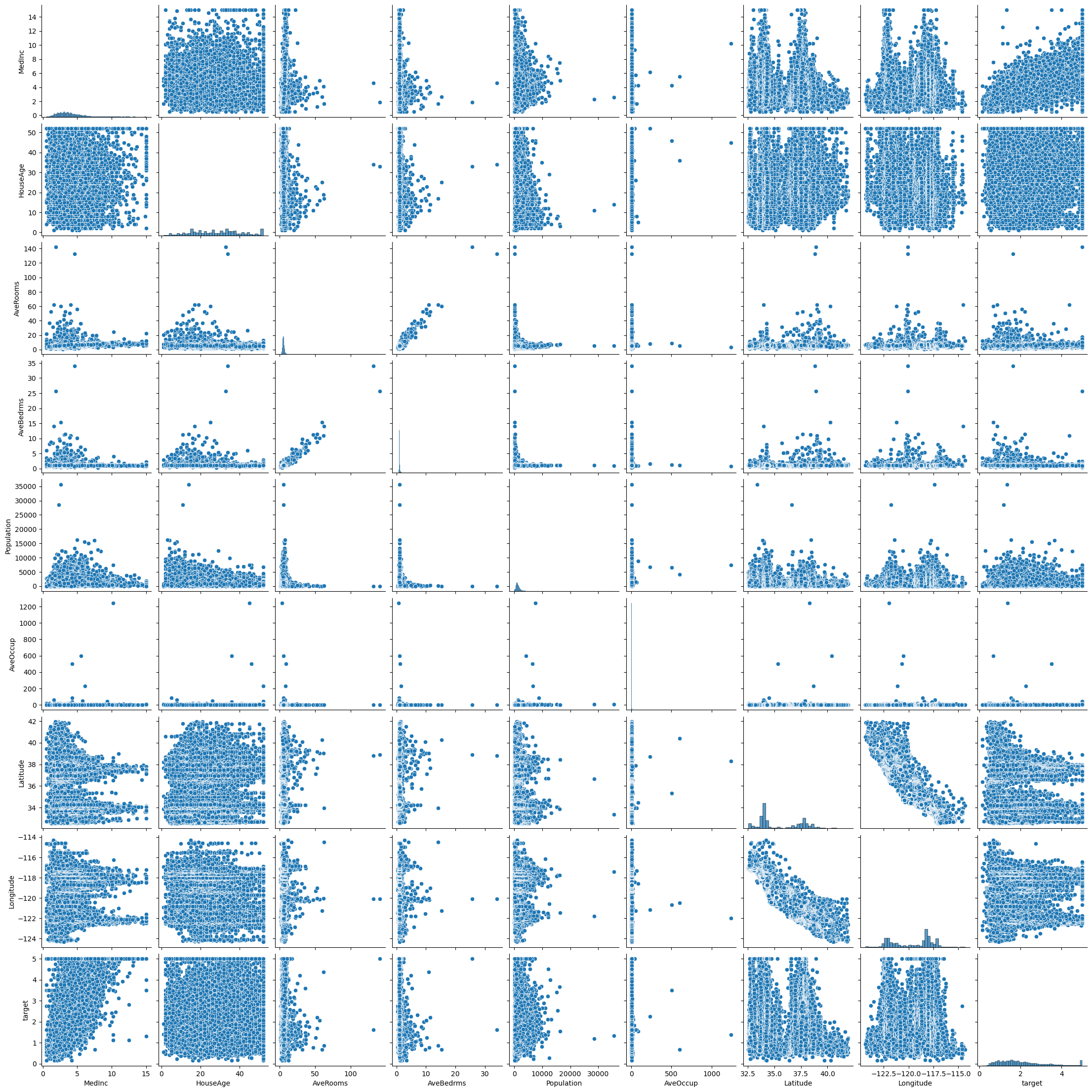
feature_names['MedInc',
'HouseAge',
'AveRooms',
'AveBedrms',
'Population',
'AveOccup',
'Latitude',
'Longitude']# Test train split and Standard Scalar
cols=feature_names
X = df[cols]
y = df['target']
X_train, X_test, y_train, y_test = train_test_split(X,y,
train_size=0.2,
random_state=42)
scalar = StandardScaler()
X_train_sc = scalar.fit_transform(X_train)
X_test_sc = scalar.transform(X_test)model = DecisionTreeRegressor(max_depth=20,random_state=42)kf = KFold(n_splits=5, shuffle=True, random_state=42)Here we need to use the negative mean squared error, because sklearn always maximizes the score!
scores = cross_val_score(model, X_train_sc, y_train, cv=kf, scoring='neg_mean_squared_error')
rmse_scores = np.sqrt(-scores)print("RMSE for each fold:", rmse_scores)
print("Mean RMSE:", rmse_scores.mean())RMSE for each fold: [0.82777432 0.80336519 0.82161843 0.82172991 0.80179882]
Mean RMSE: 0.8152573324677832Now we could play around with parameters to see which parameters give us the smallest root mean squared error?
NOTE - why might we take the square root of the MSE? This helps us interpret the magnitude of the error. MSE is error squared vs RMSE is just the error. In the example above we have an average error shown in the units of the target variable. The target variable is the median house value for California districts, expressed in hundreds of thousands of dollars ($100,000).
This tells me that we probably have some work to do! Maybe we should pick a different model or play around with the number of features.
# Maybe Try KNN???
model = KNeighborsRegressor(n_neighbors=10)
kf = KFold(n_splits=5, shuffle=True, random_state=42)
scores = cross_val_score(model, X_train_sc, y_train, cv=kf, scoring='neg_mean_squared_error')
rmse_scores = np.sqrt(-scores)
print("RMSE for each fold:", rmse_scores)
print("Mean RMSE:", rmse_scores.mean())
RMSE for each fold: [0.70952381 0.67885262 0.68315166 0.68933035 0.67586197]
Mean RMSE: 0.687344082453111Notice we are able to do all of this testing using only the training data and never looking at our final testing data!
Hyperparameter Tuning
We have talked so far about a few different types of hyperparameters:
- Number of neighbors in KNN
- Maximum depth of a decision tree
- Pruning in a decision tree
- Regularization strength (C) in logistic or linear regression
- Decision cutoff in logistic regression
To explore these values we have looped over possible numbers and then compared the training and testing values. What we saw above is that we can use cross-validation to explore parameters wihtout ever giving our model information about the testing set. Now we will see how to use built in sklearn tools to be systematic about searching parameter space for good values.
Grid Search
Given a set of possible hyperparameters, grid search evaluates all combinations using cross-validation. Lets try a grid search of the values of cpp_alpha and max depth in our decision tree regressor above.
You choose your model and then consider what hyperparameters can be plugged into that model. You create a dictionary with the possible parameter values. Then grid search tries every combination of values in a grid and uses crossvalidation to get the best possible score. The result is the best combination of values within the range your provided.
Keep in mind:
- If you get a “best” value that is on the edge of one of your ranges you may want to expand your range.
- This can be very computationally expensive depending on how many values you need to search through and how complicated your model is.
model = DecisionTreeRegressor(random_state=42)

param_grid = {
'max_depth': [2, 3, 4, 5, 6, 7, 8, 9 ,10],
'ccp_alpha': [0,0.001,0.005,0.01,0.05]
}

grid = GridSearchCV(model, param_grid, cv=10, scoring='neg_mean_squared_error')

grid.fit(X_train_sc, y_train)

print("Best parameters:", grid.best_params_)
print("Best CV score:", grid.best_score_)
Best parameters: {'ccp_alpha': 0.001, 'max_depth': 9}
Best CV score: -0.5153355581426705Now we see that the best we can do here is with ccp_alpha=0.001 and max_depth=9. BUT we are only as good as the ranges we pick.
model = DecisionTreeRegressor(random_state=42)

param_grid = {
'max_depth': [8, 9 ,10],
'ccp_alpha': [0.0015,0.002,0.0025]
}

grid = GridSearchCV(model, param_grid, cv=10, scoring='neg_mean_squared_error')

grid.fit(X_train_sc, y_train)

print("Best parameters:", grid.best_params_)
print("Best CV score:", grid.best_score_)
Best parameters: {'ccp_alpha': 0.0015, 'max_depth': 9}
Best CV score: -0.5074970912903048# My final model
model = DecisionTreeRegressor(ccp_alpha=0.0015, max_depth=9,random_state=42)
model.fit(X_train_sc,y_train)
y_pred_train = model.predict(X_train_sc)
y_pred_test = model.predict(X_test_sc)
print(f'MSE on training: {mean_squared_error(y_train,y_pred_train)}')
print(f'MSE on testing: {mean_squared_error(y_test,y_pred_test)}')MSE on training: 0.3111514699363697
MSE on testing: 0.46953543561470873Randomized Search
Rather than exhaustively trying all combinations, randomized search samples parameter combinations. This is usefull with a very large parameter space - when you have lots of hyperparameters to try. This is also typically a faster search with a good chance of hitting on a good combination of values - but it could miss the exact best combination.
model = DecisionTreeRegressor(random_state=42)

param_dist = {
'max_depth': np.arange(2,30,1),
'ccp_alpha': np.arange(0,0.05,0.0001)
}


rand_search = RandomizedSearchCV(model, param_dist, n_iter=10,
                                 cv=10,
                                 scoring='neg_mean_squared_error')

rand_search.fit(X_train_sc, y_train)

print("Best parameters:", rand_search.best_params_)
print("Best CV score:", rand_search.best_score_)
Best parameters: {'max_depth': np.int64(7), 'ccp_alpha': np.float64(0.0041)}
Best CV score: -0.5439342917275906Notice that we got some different values here from what we got in our grid search!
Avoiding Data Leakage - Pipelines
Now above we did some preprocessing before we did our cross-validation. The problem is that we learned something on the FULL training data (the standard scalar info) and then tried to do cross_validation within this data. So the validation folds actually know something about the training folds! For the most precision we should include all model preprocessing as part of a pipeline that cross-validation knows about.
Here are some things that are part of model preprocessing - the stuff we do after test-train split.
- Feature Scaling / Normalization - Standardization (StandardScaler) → mean 0, std 1
- Handling Missing Values - Filling with mean, median, mode
- Encoding Categorical Variables - One-hot encoding (OneHotEncoder)
- Feature Engineering / Transformation - Polynomial features (PolynomialFeatures) or Custom transformations derived from domain knowledge
- Dimensionality Reduction - Principal Component Analysis (PCA)
- Text / Signal Processing Tokenization, vectorization, embedding / word vector transformations
- Outlier Detection / Removal
To do this we define a pipeline!
Let’s look at the housing data again from start to finish!
X, y = fetch_california_housing(return_X_y=True)
feature_names = fetch_california_housing().feature_names

df = pd.DataFrame(X, columns=feature_names)
df["target"] = y

df| MedInc | HouseAge | AveRooms | AveBedrms | Population | AveOccup | Latitude | Longitude | target | |
|---|---|---|---|---|---|---|---|---|---|
| 0 | 8.3252 | 41.0 | 6.984127 | 1.023810 | 322.0 | 2.555556 | 37.88 | -122.23 | 4.526 |
| 1 | 8.3014 | 21.0 | 6.238137 | 0.971880 | 2401.0 | 2.109842 | 37.86 | -122.22 | 3.585 |
| 2 | 7.2574 | 52.0 | 8.288136 | 1.073446 | 496.0 | 2.802260 | 37.85 | -122.24 | 3.521 |
| 3 | 5.6431 | 52.0 | 5.817352 | 1.073059 | 558.0 | 2.547945 | 37.85 | -122.25 | 3.413 |
| 4 | 3.8462 | 52.0 | 6.281853 | 1.081081 | 565.0 | 2.181467 | 37.85 | -122.25 | 3.422 |
| ... | ... | ... | ... | ... | ... | ... | ... | ... | ... |
| 20635 | 1.5603 | 25.0 | 5.045455 | 1.133333 | 845.0 | 2.560606 | 39.48 | -121.09 | 0.781 |
| 20636 | 2.5568 | 18.0 | 6.114035 | 1.315789 | 356.0 | 3.122807 | 39.49 | -121.21 | 0.771 |
| 20637 | 1.7000 | 17.0 | 5.205543 | 1.120092 | 1007.0 | 2.325635 | 39.43 | -121.22 | 0.923 |
| 20638 | 1.8672 | 18.0 | 5.329513 | 1.171920 | 741.0 | 2.123209 | 39.43 | -121.32 | 0.847 |
| 20639 | 2.3886 | 16.0 | 5.254717 | 1.162264 | 1387.0 | 2.616981 | 39.37 | -121.24 | 0.894 |
20640 rows × 9 columns
At this point you can, and should, do so data exploration: Data Visualization, Value Counts, Descriptive Statistics, NaNs, etc.
YOU SHOULD NOT - fill in missing values with things like mean of the column or do a standard scalar which uses information about the mean and standard deviation of the column! Put this stuff in the pipeline.
The pipeline is an ordered list of tuples containingn the name and the operation that should be done.
pipe = Pipeline([
    ('scaler', StandardScaler()),
    ('model',DecisionTreeRegressor(random_state=42))
])

param_dist = {
'model__max_depth': np.arange(2,30,1),
'model__ccp_alpha': np.arange(0,0.05,0.0001)
}


rand_search_pipe = RandomizedSearchCV(pipe, param_dist, n_iter=10,
                                 cv=10,
                                 scoring='neg_mean_squared_error')

rand_search_pipe.fit(X_train_sc, y_train)

print("Best parameters:", rand_search_pipe.best_params_)
print("Best CV score:", rand_search_pipe.best_score_)
Best parameters: {'model__max_depth': np.int64(12), 'model__ccp_alpha': np.float64(0.014400000000000001)}
Best CV score: -0.6146845951141484Summary
- Cross-validation provides more reliable performance estimates.
- Hyperparameter tuning seeks values that minimize CV error.
GridSearchCVandRandomizedSearchCVautomate tuning.- Pipelines prevent data leakage.