# Some basic package imports
import os
import numpy as np
import pandas as pd

# Visualization packages
import matplotlib.pyplot as plt
import plotly.express as px
from plotly.subplots import make_subplots
import plotly.io as pio
pio.renderers.defaule = 'colab'
import seaborn as snsIntermediate Data Science
Data Aggregation and Group Operations
Intermediate Data Science
Important Information
- Email: joanna_bieri@redlands.edu
- Office Hours take place in Duke 209 – Office Hours Schedule
- Class Website
- Syllabus
Data Aggregation and Groups
Applying functions to separate groups of your data can be a critical component of data analysis. Often we have questions about how subgroups of the data differ or we might want to compute pivot tables for reporting or visualization. We are going to get more in depth into the groupby() function and really see if we can understand what it is doing and what object is returned from it. We will also see how to compute pivot tables and cross-tabulations.
Grouping
When grouping we use split-apply-combine to describe group operations.
- SPLIT - we first split the data based on one or more keys. Think about categorical values in a single column.
- APPLY - now we apply a function to each of the data subsets that we split above.
- COMBINE - finally the results of these functions are combined into a single summary output or result object.
Here is some example data
df = pd.DataFrame({"key1" : ["a", "a", None, "b", "b", "a", None],
                   "key2" : pd.Series([1, 2, 1, 2, 1, None, 1],
                                      dtype="Int64"),
                   "data1" : np.random.standard_normal(7),
                   "data2" : np.random.standard_normal(7)})
df| key1 | key2 | data1 | data2 | |
|---|---|---|---|---|
| 0 | a | 1 | 0.667991 | 0.258252 |
| 1 | a | 2 | -0.143640 | 0.316452 |
| 2 | None | 1 | -0.502239 | -0.143485 |
| 3 | b | 2 | -0.785899 | 0.383478 |
| 4 | b | 1 | 0.693085 | -1.061101 |
| 5 | a | <NA> | -0.807092 | -0.394375 |
| 6 | None | 1 | -1.021366 | -1.936547 |
What if you wanted to calculate the mean of the column data1, but on subsets or groups based on key1.
# First group the data
grouped = df["data1"].groupby(df["key1"])

# What is this object
grouped
<pandas.core.groupby.generic.SeriesGroupBy object at 0x7fede00d34d0>Notice that we can’t see our data here. This has created a python object that contains all the information we need to apply a function, but it has not actually computed anything yet. We have prepared our split.
Now we will apply a function!
grouped.sum()key1
a -0.282740
b -0.092813
Name: data1, dtype: float64We have now applied a function and combined the results into a series.
More Examples
# Calculate the mean of the data in column data1
# Group by two keys
# Results in hierarchical index
df["data1"].groupby([df["key1"], df["key2"]]).mean()
key1 key2
a 1 0.667991
2 -0.143640
b 1 0.693085
2 -0.785899
Name: data1, dtype: float64# Calculate the means of both column data1 and data2
# Group by both key1 and key2
df.groupby([df["key1"], df["key2"]]).mean()| data1 | data2 | ||
|---|---|---|---|
| key1 | key2 | ||
| a | 1 | 0.667991 | 0.258252 |
| 2 | -0.143640 | 0.316452 | |
| b | 1 | 0.693085 | -1.061101 |
| 2 | -0.785899 | 0.383478 |
# Group by key1 and then ask the size of each group
# This will automatically drop NaNs
df.groupby('key1').size()
key1
a 3
b 2
dtype: int64df.groupby('key1',dropna=False).size()key1
a 3
b 2
NaN 2
dtype: int64# Count the number of nonnull values
df.groupby('key1').count()| key2 | data1 | data2 | |
|---|---|---|---|
| key1 | |||
| a | 2 | 3 | 3 |
| b | 2 | 2 | 2 |
You Try
Try applying some other function that are available to the groupby object. See if you can figure out what the function is doing. To see all the possible functions try groupby. and then hit tab!
# Your code hereIterating over Groups
You can iterate over the group object returned from groupby().
grouped = df["data1"].groupby(df["key1"])

for g in grouped:
    print(g[0])
    display(g[1])
a
b0 0.667991
1 -0.143640
5 -0.807092
Name: data1, dtype: float643 -0.785899
4 0.693085
Name: data1, dtype: float64You can see that each thing in our grouped object is a tuple. The first entry in the tuple is the group name (or category) the second object is a Series or a DataFrame depending on the number of columns sent in.
grouped = df[["data1","data2"]].groupby(df["key1"])

for g in grouped:
    print(g[0])
    display(g[1])
a
b| data1 | data2 | |
|---|---|---|
| 0 | 0.667991 | 0.258252 |
| 1 | -0.143640 | 0.316452 |
| 5 | -0.807092 | -0.394375 |
| data1 | data2 | |
|---|---|---|
| 3 | -0.785899 | 0.383478 |
| 4 | 0.693085 | -1.061101 |
# If you group by two keys, your group names have two values.
grouped = df[["data1","data2"]].groupby([df["key1"],df["key2"]])

for g in grouped:
    print(g[0])
    display(g[1])
('a', np.int64(1))
('a', np.int64(2))
('b', np.int64(1))
('b', np.int64(2))| data1 | data2 | |
|---|---|---|
| 0 | 0.667991 | 0.258252 |
| data1 | data2 | |
|---|---|---|
| 1 | -0.14364 | 0.316452 |
| data1 | data2 | |
|---|---|---|
| 4 | 0.693085 | -1.061101 |
| data1 | data2 | |
|---|---|---|
| 3 | -0.785899 | 0.383478 |
Column vs Row Grouping
By default groups are created on the axis=‘index’ meaning that it is breaking up the rows into groups based on labels in a column. But we could break up columns based on values in a row.
Here is an example where we group the data based on column names.
- We take the transpose of the dataframe.
- Here we send in a dictionary that maps the values found in the index to either key or data.
- The groupby now splits based on our old column names.
df.T| 0 | 1 | 2 | 3 | 4 | 5 | 6 | |
|---|---|---|---|---|---|---|---|
| key1 | a | a | None | b | b | a | None |
| key2 | 1 | 2 | 1 | 2 | 1 | <NA> | 1 |
| data1 | 0.667991 | -0.14364 | -0.502239 | -0.785899 | 0.693085 | -0.807092 | -1.021366 |
| data2 | 0.258252 | 0.316452 | -0.143485 | 0.383478 | -1.061101 | -0.394375 | -1.936547 |
# Here we map the names found in the index
# To new names - we will group on the new names.
mapping = {"key1": "key", "key2": "key",
            "data1": "data", "data2": "data"}

grouped = df.T.groupby(mapping)

for g in grouped:
    print(g[0])
    display(g[1])
data
key| 0 | 1 | 2 | 3 | 4 | 5 | 6 | |
|---|---|---|---|---|---|---|---|
| data1 | 0.667991 | -0.14364 | -0.502239 | -0.785899 | 0.693085 | -0.807092 | -1.021366 |
| data2 | 0.258252 | 0.316452 | -0.143485 | 0.383478 | -1.061101 | -0.394375 | -1.936547 |
| 0 | 1 | 2 | 3 | 4 | 5 | 6 | |
|---|---|---|---|---|---|---|---|
| key1 | a | a | None | b | b | a | None |
| key2 | 1 | 2 | 1 | 2 | 1 | <NA> | 1 |
Grouping with Functions
You can also use python functions to specify groups.
For example, in the data below we have information about different people. What if you wanted to group a data set based on the length of their name. You can do that!
people = pd.DataFrame(np.random.standard_normal((5, 5)),
                      columns=["a", "b", "c", "d", "e"],
                      index=["Joe", "Steve", "Wanda", "Jill", "Trey"])
people.iloc[2:3, [1, 2]] = np.nan # Add a few NA values
people| a | b | c | d | e | |
|---|---|---|---|---|---|
| Joe | -0.022397 | -0.502856 | -0.004511 | -1.985540 | 0.186960 |
| Steve | 0.437526 | 0.467422 | 0.195933 | -0.642973 | 1.054600 |
| Wanda | -0.819018 | NaN | NaN | 1.719955 | -0.249791 |
| Jill | 0.047468 | 0.051260 | 0.867313 | -0.664157 | -1.172044 |
| Trey | 0.636158 | 2.495864 | -1.547932 | -0.117629 | -1.861339 |
grouped = people.groupby(len)

for g in grouped:
    print(g[0])
    display(g[1])
3
4
5| a | b | c | d | e | |
|---|---|---|---|---|---|
| Joe | -0.022397 | -0.502856 | -0.004511 | -1.98554 | 0.18696 |
| a | b | c | d | e | |
|---|---|---|---|---|---|
| Jill | 0.047468 | 0.051260 | 0.867313 | -0.664157 | -1.172044 |
| Trey | 0.636158 | 2.495864 | -1.547932 | -0.117629 | -1.861339 |
| a | b | c | d | e | |
|---|---|---|---|---|---|
| Steve | 0.437526 | 0.467422 | 0.195933 | -0.642973 | 1.054600 |
| Wanda | -0.819018 | NaN | NaN | 1.719955 | -0.249791 |
You Try
Read in the macro data - same as last class - just run the code below.
Then group the data by year and apply a function that makes sense with this data. Something like mean, max, min, etc…
Finally plot the resulting time-series data. For example, the average cpi over time.
macro = pd.read_csv("data/macrodata.csv")
data = macro[["year","quarter","cpi", "m1", "tbilrate", "unemp"]]
# Your code hereData Aggregation
Data aggregation is when you take an array (or list) of values and apply a transformation that produces a single scalar output. Think about a list of grades and then taking an average.
Functions that are optimized for the groupby() method
| Aggregation Function | Description | Example Usage |
|---|---|---|
sum |
Sum of values (ignores NaN) | df.groupby("col")["val"].sum() |
mean |
Mean (average) of values (ignores NaN) | df.groupby("col")["val"].mean() |
median |
Median (50th percentile) | df.groupby("col")["val"].median() |
min |
Minimum value | df.groupby("col")["val"].min() |
max |
Maximum value | df.groupby("col")["val"].max() |
count |
Count of non-NaN values | df.groupby("col")["val"].count() |
size |
Count of all rows (including NaN) | df.groupby("col").size() |
std |
Standard deviation (ddof=1 by default) | df.groupby("col")["val"].std() |
var |
Variance (ddof=1 by default) | df.groupby("col")["val"].var() |
prod |
Product of values | df.groupby("col")["val"].prod() |
first |
First non-NaN value in group | df.groupby("col")["val"].first() |
last |
Last non-NaN value in group | df.groupby("col")["val"].last() |
nunique |
Number of distinct values | df.groupby("col")["val"].nunique() |
Functions that can be applied to groupby but are a bit slower
| Aggregation Function | Description | Example Usage | Notes |
|---|---|---|---|
mode |
Most frequent value(s) in group | df.groupby("col")["val"].agg(pd.Series.mode) |
Can return multiple values per group |
skew |
Sample skewness of distribution | df.groupby("col")["val"].skew() |
Slower, especially on large groups |
kurt / kurtosis |
Kurtosis (tailedness of distribution) | df.groupby("col")["val"].kurt() |
Not Cython-optimized |
quantile |
Value at given quantile (e.g. 0.25, 0.75) | df.groupby("col")["val"].quantile(0.25) |
Flexible but slower |
sem |
Standard error of the mean | df.groupby("col")["val"].sem() |
Based on std / sqrt(n) |
mad |
Mean absolute deviation | df.groupby("col")["val"].mad() |
Not Cythonized |
describe |
Multiple summary stats at once | df.groupby("col")["val"].describe() |
Returns count, mean, std, min, etc. |
| Custom functions | Any user-defined aggregation (via .apply) |
df.groupby("col")["val"].apply(func) |
Flexible but usually much slower |
Now sometimes you want to apply muptliple functions to a single grouped object. One way to do this is with the .agg() function. Lets read in the tips data we have seen before:
tips = pd.read_csv("data/tips.csv")
tips.head()| total_bill | tip | smoker | day | time | size | |
|---|---|---|---|---|---|---|
| 0 | 16.99 | 1.01 | No | Sun | Dinner | 2 |
| 1 | 10.34 | 1.66 | No | Sun | Dinner | 3 |
| 2 | 21.01 | 3.50 | No | Sun | Dinner | 3 |
| 3 | 23.68 | 3.31 | No | Sun | Dinner | 2 |
| 4 | 24.59 | 3.61 | No | Sun | Dinner | 4 |
Now lets say that we want to understand the tip percentage from different groups: smokers vs nonsmokers, vs day of the week. Maybe you want to know the average and standard deviation of the tip percentage and you want to define a calculation of your own called max_to_min that calculates the difference between the max and min percent.
# First we have to add the percentage to the data
tips["tip_pct"] = tips["tip"] / tips["total_bill"]
# Now we can define our own custom function
def max_to_min(arr):
return arr.max() - arr.min()# Next lets group the data
grouped = tips.groupby(["day", "smoker"])# And finally apply the functions using the .agg()
functions = ["mean", "std", max_to_min]
agg_data = grouped['tip_pct'].agg(functions)
agg_data| mean | std | max_to_min | ||
|---|---|---|---|---|
| day | smoker | |||
| Fri | No | 0.151650 | 0.028123 | 0.067349 |
| Yes | 0.174783 | 0.051293 | 0.159925 | |
| Sat | No | 0.158048 | 0.039767 | 0.235193 |
| Yes | 0.147906 | 0.061375 | 0.290095 | |
| Sun | No | 0.160113 | 0.042347 | 0.193226 |
| Yes | 0.187250 | 0.154134 | 0.644685 | |
| Thur | No | 0.160298 | 0.038774 | 0.193350 |
| Yes | 0.163863 | 0.039389 | 0.151240 |
This is a case where I would use pandas .plot()
# Graph the results
agg_data.plot.bar()
plt.grid()
plt.show()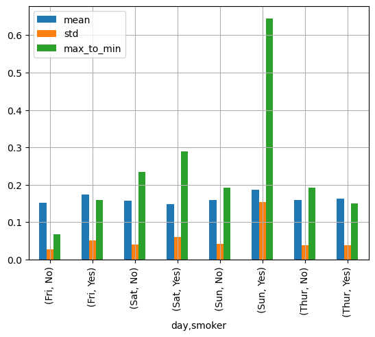
# You can also return the data without the groups as and index
# just use the as_index=False command
grouped2 = tips.groupby(["day", "smoker"],as_index=False)
functions = ["mean", "std", max_to_min]
agg_data2 = grouped2['tip_pct'].agg(functions)
agg_data2| day | smoker | mean | std | max_to_min | |
|---|---|---|---|---|---|
| 0 | Fri | No | 0.151650 | 0.028123 | 0.067349 |
| 1 | Fri | Yes | 0.174783 | 0.051293 | 0.159925 |
| 2 | Sat | No | 0.158048 | 0.039767 | 0.235193 |
| 3 | Sat | Yes | 0.147906 | 0.061375 | 0.290095 |
| 4 | Sun | No | 0.160113 | 0.042347 | 0.193226 |
| 5 | Sun | Yes | 0.187250 | 0.154134 | 0.644685 |
| 6 | Thur | No | 0.160298 | 0.038774 | 0.193350 |
| 7 | Thur | Yes | 0.163863 | 0.039389 | 0.151240 |
From this example hopefully you can see how powerful grouping and aggregating can be in quickly comparing parts of your dataset!
You Try
What happens when you run the following command using the tip data above? Can you predict what the output will be before you run the code? Then run the code and explain the results. Finally make a plot - your choice on the type.
grouped = tips.groupby(["day", "smoker","time"])
functions = ["count", "mean", "max"]
result = grouped[["tip_pct", "total_bill"]].agg(functions)
result
# Your code hereQuantile and Bucket Analysis
We have seen some functions that can help us to cut our data into buckets, pd.cut() for example. Another similar function is pd.qcut() which divides your data into sample quantiles. You can use these functions on grouped data.
Below we will use .qcut() to get quartile categories and then group by the quartiles. Finally we can aggregate over that data.
quartiles = pd.qcut(tips['total_bill'],4)
tips['quartiles'] = quartiles
tips.head()| total_bill | tip | smoker | day | time | size | tip_pct | quartiles | |
|---|---|---|---|---|---|---|---|---|
| 0 | 16.99 | 1.01 | No | Sun | Dinner | 2 | 0.059447 | (13.348, 17.795] |
| 1 | 10.34 | 1.66 | No | Sun | Dinner | 3 | 0.160542 | (3.069, 13.348] |
| 2 | 21.01 | 3.50 | No | Sun | Dinner | 3 | 0.166587 | (17.795, 24.127] |
| 3 | 23.68 | 3.31 | No | Sun | Dinner | 2 | 0.139780 | (17.795, 24.127] |
| 4 | 24.59 | 3.61 | No | Sun | Dinner | 4 | 0.146808 | (24.127, 50.81] |
grouped = tips['total_bill'].groupby(tips['quartiles'])
grouped.agg(["count","max","min","mean"])| count | max | min | mean | |
|---|---|---|---|---|
| quartiles | ||||
| (3.069, 13.348] | 61 | 13.28 | 3.07 | 10.691967 |
| (13.348, 17.795] | 61 | 17.78 | 13.37 | 15.618689 |
| (17.795, 24.127] | 61 | 24.08 | 17.81 | 20.498525 |
| (24.127, 50.81] | 61 | 50.81 | 24.27 | 32.334590 |
More Examples of using groupby()
Filling Missing Values
states = ["Ohio", "New York", "Vermont", "Florida",
          "Oregon", "Nevada", "California", "Idaho"]
location = ["East", "East", "East", "East",
             "West", "West", "West", "West"]
data = pd.DataFrame({'Data':np.random.standard_normal(8),
                     'Location':location},
                    index=states)

# Add some NaNs
for s in ["Vermont", "Nevada", "Idaho"]:
    data.loc[s, "Data"] = np.nan
data| Data | Location | |
|---|---|---|
| Ohio | 0.849264 | East |
| New York | 0.083113 | East |
| Vermont | NaN | East |
| Florida | 1.207980 | East |
| Oregon | -0.085424 | West |
| Nevada | NaN | West |
| California | -0.739081 | West |
| Idaho | NaN | West |
What if we wanted to fill these NaNs, but with different values based on whether they are in the east or west. Maybe we want to average the east and west values and use that number to fill the NaNs.
# Define a function that will return the fill value
def fill_mean(group):
    return group.fillna(group.mean())

# We group by location
grouped = data.groupby('Location')
# Then fill in the NANs with the averages of the group
grouped.apply(fill_mean)| Data | ||
|---|---|---|
| Location | ||
| East | Ohio | 0.849264 |
| New York | 0.083113 | |
| Vermont | 0.713452 | |
| Florida | 1.207980 | |
| West | Oregon | -0.085424 |
| Nevada | -0.412252 | |
| California | -0.739081 | |
| Idaho | -0.412252 |
Groupwise Linear Regression
We talked about linear regression in DATA101 and DATA100. It is a way to fit a straight line to some given data.
We will use sklearn to do this. If you don’t have it installed, you should install it.
# !conda install -y scikit-learn# Get some data
close_px = pd.read_csv("data/stock_px.csv", parse_dates=True,
index_col=0)
# The .info() command gives you information about the data
# Including data types and number of nonnulls
close_px.info()<class 'pandas.core.frame.DataFrame'>
DatetimeIndex: 2214 entries, 2003-01-02 to 2011-10-14
Data columns (total 4 columns):
# Column Non-Null Count Dtype
--- ------ -------------- -----
0 AAPL 2214 non-null float64
1 MSFT 2214 non-null float64
2 XOM 2214 non-null float64
3 SPX 2214 non-null float64
dtypes: float64(4)
memory usage: 86.5 KBclose_px.head()| AAPL | MSFT | XOM | SPX | |
|---|---|---|---|---|
| 2003-01-02 | 7.40 | 21.11 | 29.22 | 909.03 |
| 2003-01-03 | 7.45 | 21.14 | 29.24 | 908.59 |
| 2003-01-06 | 7.45 | 21.52 | 29.96 | 929.01 |
| 2003-01-07 | 7.43 | 21.93 | 28.95 | 922.93 |
| 2003-01-08 | 7.28 | 21.31 | 28.83 | 909.93 |
# Lets group the data by year
# First confirm that the index values are dates
first_index = close_px.index[0]
print(first_index)
print(type(first_index))
2003-01-02 00:00:00
<class 'pandas._libs.tslibs.timestamps.Timestamp'># This is a timestamp object
# You can do first_index. and press tab to see all the options
print(first_index.year)
print(first_index.month)
print(first_index.month_name())
print(first_index.day)
print(first_index.day_name())2003
1
January
2
Thursday# So first write a function that will return the year
def get_year(x):
return x.year
# Then group by the year
by_year = close_px.groupby(get_year)from sklearn.linear_model import LinearRegression
# Define a liner regression and return intercept and slope
def regress(data,xvars,yvar):
X = data[xvars]
y = data[yvar]
LM = LinearRegression()
LM.fit(X, y)
slope = LM.coef_[0]
intercept = LM.intercept_
return intercept, slope
# Apply the linear regression to the groups
by_year.apply(regress,yvar='AAPL',xvars=['SPX'])2003 (-8.58984966958583, 0.018505966710274123)
2004 (-132.12116289682774, 0.1325654494610963)
2005 (-299.5951029082234, 0.28683118762773924)
2006 (-133.18691255199056, 0.15566846429728873)
2007 (-432.9175504440354, 0.37990617598041215)
2008 (-36.33814322777991, 0.1461565642803874)
2009 (-164.38487241406185, 0.3282529241664158)
2010 (-210.84981430613925, 0.41290045011855553)
2011 (603.8769113704016, -0.1938338932016932)
dtype: objectPivot Tables and Cross-Tabulation
Pivot Table
Pivot tables are often found in spreadsheet programs and are a way to summarize data. We have seen the .pivot operation as a way to wrangle the data. Here we will look at the pivot_table() method. The results in many cases can be produced using the groupby function, but this acts as a shortcut and can add partial totals or margins to the data.
# Lets use the same tips data that we loaded in above
tips = pd.read_csv("data/tips.csv")
tips["tip_pct"] = tips["tip"] / tips["total_bill"]
tips.head()| total_bill | tip | smoker | day | time | size | tip_pct | |
|---|---|---|---|---|---|---|---|
| 0 | 16.99 | 1.01 | No | Sun | Dinner | 2 | 0.059447 |
| 1 | 10.34 | 1.66 | No | Sun | Dinner | 3 | 0.160542 |
| 2 | 21.01 | 3.50 | No | Sun | Dinner | 3 | 0.166587 |
| 3 | 23.68 | 3.31 | No | Sun | Dinner | 2 | 0.139780 |
| 4 | 24.59 | 3.61 | No | Sun | Dinner | 4 | 0.146808 |
tips.pivot_table(index=["day", "smoker"],
values=["size", "tip", "tip_pct", "total_bill"])| size | tip | tip_pct | total_bill | ||
|---|---|---|---|---|---|
| day | smoker | ||||
| Fri | No | 2.250000 | 2.812500 | 0.151650 | 18.420000 |
| Yes | 2.066667 | 2.714000 | 0.174783 | 16.813333 | |
| Sat | No | 2.555556 | 3.102889 | 0.158048 | 19.661778 |
| Yes | 2.476190 | 2.875476 | 0.147906 | 21.276667 | |
| Sun | No | 2.929825 | 3.167895 | 0.160113 | 20.506667 |
| Yes | 2.578947 | 3.516842 | 0.187250 | 24.120000 | |
| Thur | No | 2.488889 | 2.673778 | 0.160298 | 17.113111 |
| Yes | 2.352941 | 3.030000 | 0.163863 | 19.190588 |
NOTE by default the pivot table returns the mean()
We could have done the same operation with groupby!
Arguments you might want to pass into the pivot_table() function:
- index – the values that you are grouping by
- values – the numbers you are aggregating
- columns – categories to subset the columns - adding extra columns to the output
- margin=True – include the margin or the value for the whole
- aggfunc – aggregation function if you want something other than mean.
- fill_value – what you want to full if the computation runs into a NaN
Here are some examples:
tips.pivot_table(index=["time", "day"], columns="smoker",
values=["tip_pct", "size"], margins=True)| size | tip_pct | ||||||
|---|---|---|---|---|---|---|---|
| smoker | No | Yes | All | No | Yes | All | |
| time | day | ||||||
| Dinner | Fri | 2.000000 | 2.222222 | 2.166667 | 0.139622 | 0.165347 | 0.158916 |
| Sat | 2.555556 | 2.476190 | 2.517241 | 0.158048 | 0.147906 | 0.153152 | |
| Sun | 2.929825 | 2.578947 | 2.842105 | 0.160113 | 0.187250 | 0.166897 | |
| Thur | 2.000000 | NaN | 2.000000 | 0.159744 | NaN | 0.159744 | |
| Lunch | Fri | 3.000000 | 1.833333 | 2.000000 | 0.187735 | 0.188937 | 0.188765 |
| Thur | 2.500000 | 2.352941 | 2.459016 | 0.160311 | 0.163863 | 0.161301 | |
| All | 2.668874 | 2.408602 | 2.569672 | 0.159328 | 0.163196 | 0.160803 | |
tips.pivot_table(index=["time", "day"], columns="smoker",
values=["tip_pct", "size"], aggfunc="max")| size | tip_pct | ||||
|---|---|---|---|---|---|
| smoker | No | Yes | No | Yes | |
| time | day | ||||
| Dinner | Fri | 2.0 | 4.0 | 0.155625 | 0.263480 |
| Sat | 4.0 | 5.0 | 0.291990 | 0.325733 | |
| Sun | 6.0 | 5.0 | 0.252672 | 0.710345 | |
| Thur | 2.0 | NaN | 0.159744 | NaN | |
| Lunch | Fri | 3.0 | 2.0 | 0.187735 | 0.259314 |
| Thur | 6.0 | 4.0 | 0.266312 | 0.241255 | |
tips.pivot_table(index=["time", "size", "smoker"], columns="day",
values="tip_pct")| day | Fri | Sat | Sun | Thur | ||
|---|---|---|---|---|---|---|
| time | size | smoker | ||||
| Dinner | 1 | No | NaN | 0.137931 | NaN | NaN |
| Yes | NaN | 0.325733 | NaN | NaN | ||
| 2 | No | 0.139622 | 0.162705 | 0.168859 | 0.159744 | |
| Yes | 0.171297 | 0.148668 | 0.207893 | NaN | ||
| 3 | No | NaN | 0.154661 | 0.152663 | NaN | |
| Yes | NaN | 0.144995 | 0.152660 | NaN | ||
| 4 | No | NaN | 0.150096 | 0.148143 | NaN | |
| Yes | 0.117750 | 0.124515 | 0.193370 | NaN | ||
| 5 | No | NaN | NaN | 0.206928 | NaN | |
| Yes | NaN | 0.106572 | 0.065660 | NaN | ||
| 6 | No | NaN | NaN | 0.103799 | NaN | |
| Lunch | 1 | No | NaN | NaN | NaN | 0.181728 |
| Yes | 0.223776 | NaN | NaN | NaN | ||
| 2 | No | NaN | NaN | NaN | 0.166005 | |
| Yes | 0.181969 | NaN | NaN | 0.158843 | ||
| 3 | No | 0.187735 | NaN | NaN | 0.084246 | |
| Yes | NaN | NaN | NaN | 0.204952 | ||
| 4 | No | NaN | NaN | NaN | 0.138919 | |
| Yes | NaN | NaN | NaN | 0.155410 | ||
| 5 | No | NaN | NaN | NaN | 0.121389 | |
| 6 | No | NaN | NaN | NaN | 0.173706 |
tips.pivot_table(index=["time", "size", "smoker"], columns="day",
values="tip_pct",fill_value=0)| day | Fri | Sat | Sun | Thur | ||
|---|---|---|---|---|---|---|
| time | size | smoker | ||||
| Dinner | 1 | No | 0.000000 | 0.137931 | 0.000000 | 0.000000 |
| Yes | 0.000000 | 0.325733 | 0.000000 | 0.000000 | ||
| 2 | No | 0.139622 | 0.162705 | 0.168859 | 0.159744 | |
| Yes | 0.171297 | 0.148668 | 0.207893 | 0.000000 | ||
| 3 | No | 0.000000 | 0.154661 | 0.152663 | 0.000000 | |
| Yes | 0.000000 | 0.144995 | 0.152660 | 0.000000 | ||
| 4 | No | 0.000000 | 0.150096 | 0.148143 | 0.000000 | |
| Yes | 0.117750 | 0.124515 | 0.193370 | 0.000000 | ||
| 5 | No | 0.000000 | 0.000000 | 0.206928 | 0.000000 | |
| Yes | 0.000000 | 0.106572 | 0.065660 | 0.000000 | ||
| 6 | No | 0.000000 | 0.000000 | 0.103799 | 0.000000 | |
| Lunch | 1 | No | 0.000000 | 0.000000 | 0.000000 | 0.181728 |
| Yes | 0.223776 | 0.000000 | 0.000000 | 0.000000 | ||
| 2 | No | 0.000000 | 0.000000 | 0.000000 | 0.166005 | |
| Yes | 0.181969 | 0.000000 | 0.000000 | 0.158843 | ||
| 3 | No | 0.187735 | 0.000000 | 0.000000 | 0.084246 | |
| Yes | 0.000000 | 0.000000 | 0.000000 | 0.204952 | ||
| 4 | No | 0.000000 | 0.000000 | 0.000000 | 0.138919 | |
| Yes | 0.000000 | 0.000000 | 0.000000 | 0.155410 | ||
| 5 | No | 0.000000 | 0.000000 | 0.000000 | 0.121389 | |
| 6 | No | 0.000000 | 0.000000 | 0.000000 | 0.173706 |
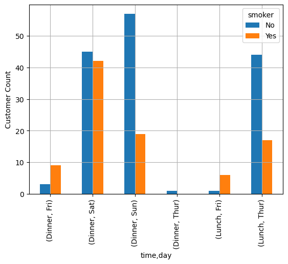
Crosstab
Cross tabulation is a type of pivot table that returns frequency observations. You can very quickly reach into your data and get counts of the number of observations that fall into each subset.
cdata = pd.crosstab([tips["time"], tips["day"]], tips["smoker"])
cdata| smoker | No | Yes | |
|---|---|---|---|
| time | day | ||
| Dinner | Fri | 3 | 9 |
| Sat | 45 | 42 | |
| Sun | 57 | 19 | |
| Thur | 1 | 0 | |
| Lunch | Fri | 1 | 6 |
| Thur | 44 | 17 |
cdata.plot.bar()
plt.grid()
plt.ylabel('Customer Count')
plt.show()