# Some basic package imports
import os
import numpy as np
import pandas as pd

# Visualization packages
import matplotlib.pyplot as plt
import plotly.express as px
from plotly.subplots import make_subplots
import plotly.io as pio
pio.renderers.defaule = 'colab'
import seaborn as snsIntermediate Data Science
Time Series Data
Intermediate Data Science
Important Information
- Email: joanna_bieri@redlands.edu
- Office Hours take place in Duke 209 – Office Hours Schedule
- Class Website
- Syllabus
Time Series Data
Time series are a form of data that are common in many fields: Economics, Finance, Ecology, Neuroscience, Physics, and Applied Math. Any data that is recorded at many points over time, with a certain frequency of observations, is time series data. Time plays an important role in the data - maybe you want to know how observations change over time.
- Fixed Frequency observations are recorded at a fixed interval. The intervals are regular and time steps consistent.
- Irregular observations do not have a fixed interval, although time is recorded and could be important to your analysis.
There are many ways that you might mark time series data:
- Timestamps time marked by recording specific instants in time.
- Fixed Periods time marked by recording the month or the year.
- Intervals of Time mark both a start and end timestamp.
- Experimental or Elapsed Time time as recorded relative to a start time.
We will mostly explore timestamps, since the other types can usually be converted into timestamps.
Date and Time Tools
We will start by exploring tools that are available for interacting with dates and times. We will look at the datetime package.
from datetime import datetime# Lets look at how time is recorded
now = datetime.now()
print(now)2025-09-30 14:00:51.845676We see the format is year, month, day, hour, minute, second, microsecond. We can access items from this datetime object. Try now. and press the tab button!
now.year2025now.day30now.month9Once you have a datetime object you can do operations like addition and subtraction.
How long have you been alive?
my_birthday = datetime(1979,2,7)
my_birthday
datetime.datetime(1979, 2, 7, 0, 0)my_life = now-my_birthday
my_lifedatetime.timedelta(days=17037, seconds=50451, microseconds=845676)You Try
Write a python function that takes as an input a birth date and outputs how old the person is in just years, by using the datetime functionality.
# Your code hereYou can add or subtract a timedelta to shift a datetime object or create a series of datetimes.
from datetime import timedelta
# timedelta(days=0, seconds=0, microseconds=0, milliseconds=0, minutes=0, hours=0, weeks=0)

start = datetime(2025,9,3,1,15)
print(start)
delta = timedelta(hours=1,minutes=5)
print(delta)
print(start+delta)
2025-09-03 01:15:00
1:05:00
2025-09-03 02:20:00# You can quickly generate lists of time data
delta = timedelta(days=1)
days_of_year = [datetime(2025,1,1)]
for i in range(30):
days_of_year.append(days_of_year[-1]+delta)days_of_year[datetime.datetime(2025, 1, 1, 0, 0),
datetime.datetime(2025, 1, 2, 0, 0),
datetime.datetime(2025, 1, 3, 0, 0),
datetime.datetime(2025, 1, 4, 0, 0),
datetime.datetime(2025, 1, 5, 0, 0),
datetime.datetime(2025, 1, 6, 0, 0),
datetime.datetime(2025, 1, 7, 0, 0),
datetime.datetime(2025, 1, 8, 0, 0),
datetime.datetime(2025, 1, 9, 0, 0),
datetime.datetime(2025, 1, 10, 0, 0),
datetime.datetime(2025, 1, 11, 0, 0),
datetime.datetime(2025, 1, 12, 0, 0),
datetime.datetime(2025, 1, 13, 0, 0),
datetime.datetime(2025, 1, 14, 0, 0),
datetime.datetime(2025, 1, 15, 0, 0),
datetime.datetime(2025, 1, 16, 0, 0),
datetime.datetime(2025, 1, 17, 0, 0),
datetime.datetime(2025, 1, 18, 0, 0),
datetime.datetime(2025, 1, 19, 0, 0),
datetime.datetime(2025, 1, 20, 0, 0),
datetime.datetime(2025, 1, 21, 0, 0),
datetime.datetime(2025, 1, 22, 0, 0),
datetime.datetime(2025, 1, 23, 0, 0),
datetime.datetime(2025, 1, 24, 0, 0),
datetime.datetime(2025, 1, 25, 0, 0),
datetime.datetime(2025, 1, 26, 0, 0),
datetime.datetime(2025, 1, 27, 0, 0),
datetime.datetime(2025, 1, 28, 0, 0),
datetime.datetime(2025, 1, 29, 0, 0),
datetime.datetime(2025, 1, 30, 0, 0),
datetime.datetime(2025, 1, 31, 0, 0)]Converting Strings
Often when you read in data from a .csv the data will be in the string format. You can go back and forth between datetime objects and strings.
dt = datetime(2000,1,1)

# The str() command can convert data into strings
str(dt)
'2000-01-01 00:00:00'# You can also format the strings
'''
%Y year
%y two digit year
%m month
%d day
There are lots of these! - see book pate 359
'''
dt.strftime("%m-%d-%Y")'01-01-2000'# Start with a string
str_date = '1-1-2000'
# You have to use the string formatting commands to tell date time how the string is formatted
# so it can strip out the parts correctly
datetime.strptime(str_date, "%m-%d-%Y")datetime.datetime(2000, 1, 1, 0, 0)Time Series Basics
We will load in some weather data so we can explore how to deal with time series data. We will stet the index to be time series data so that we can explore how we might “slice” or subset time.
import kagglehub

# Download latest version
path = kagglehub.dataset_download("parthdande/timeseries-weather-dataset")

print("Path to dataset files:", path)

print(os.listdir(path))
Warning: Looks like you're using an outdated `kagglehub` version (installed: 0.3.8), please consider upgrading to the latest version (0.3.13).
Path to dataset files: /home/bellajagu/.cache/kagglehub/datasets/parthdande/timeseries-weather-dataset/versions/2
['Weather_dataset.csv', 'Weather_Data_1980_2024(hourly).csv']df = pd.read_csv(path+'/'+'Weather_Data_1980_2024(hourly).csv')
df.head(5)| time | temperature | relative_humidity | dew_point | precipitation (mm) | rain (mm) | snowfall (cm) | pressure_msl (hPa) | surface_pressure (hPa) | cloud_cover (%) | cloud_cover_low (%) | cloud_cover_mid (%) | cloud_cover_high (%) | vapour_pressure_deficit (kPa) | wind_speed_10m (km/h) | wind_direction | is_Day | |
|---|---|---|---|---|---|---|---|---|---|---|---|---|---|---|---|---|---|
| 0 | 1980-01-01T00:00 | 12.7 | 83 | 10.0 | 0.0 | 0.0 | 0 | 1012.8 | 945.1 | 1 | 1 | 0 | 0 | 0.25 | 7.5 | 235 | 0 |
| 1 | 1980-01-01T01:00 | 12.9 | 82 | 9.9 | 0.0 | 0.0 | 0 | 1012.2 | 944.5 | 4 | 4 | 0 | 0 | 0.26 | 7.9 | 231 | 0 |
| 2 | 1980-01-01T02:00 | 13.2 | 82 | 10.2 | 0.0 | 0.0 | 0 | 1012.3 | 944.7 | 13 | 14 | 0 | 0 | 0.27 | 7.5 | 235 | 1 |
| 3 | 1980-01-01T03:00 | 15.9 | 78 | 12.0 | 0.0 | 0.0 | 0 | 1013.5 | 946.4 | 23 | 26 | 0 | 0 | 0.40 | 6.6 | 248 | 1 |
| 4 | 1980-01-01T04:00 | 19.4 | 67 | 13.1 | 0.0 | 0.0 | 0 | 1014.6 | 948.2 | 9 | 10 | 0 | 0 | 0.75 | 8.7 | 265 | 1 |
# Notice that the objects in the time column are strings
df['time'].iloc[0]'1980-01-01T00:00'# Change the times to datetime objects
# Save them as the index for the data frame.
def string_to_time(x):
'''
A function to return a datetime striped from the format:
'1980-01-01T00:00'
'''
return datetime.strptime(x,'%Y-%m-%dT%H:%M')
# Set the index using the time column and a lambda
df.index = df['time'].apply(lambda x: string_to_time(x))
# Convert the time to datetime
df['time'] = df['time'].apply(lambda x: string_to_time(x))
df| time | temperature | relative_humidity | dew_point | precipitation (mm) | rain (mm) | snowfall (cm) | pressure_msl (hPa) | surface_pressure (hPa) | cloud_cover (%) | cloud_cover_low (%) | cloud_cover_mid (%) | cloud_cover_high (%) | vapour_pressure_deficit (kPa) | wind_speed_10m (km/h) | wind_direction | is_Day | |
|---|---|---|---|---|---|---|---|---|---|---|---|---|---|---|---|---|---|
| time | |||||||||||||||||
| 1980-01-01 00:00:00 | 1980-01-01 00:00:00 | 12.7 | 83 | 10.0 | 0.0 | 0.0 | 0 | 1012.8 | 945.1 | 1 | 1 | 0 | 0 | 0.25 | 7.5 | 235 | 0 |
| 1980-01-01 01:00:00 | 1980-01-01 01:00:00 | 12.9 | 82 | 9.9 | 0.0 | 0.0 | 0 | 1012.2 | 944.5 | 4 | 4 | 0 | 0 | 0.26 | 7.9 | 231 | 0 |
| 1980-01-01 02:00:00 | 1980-01-01 02:00:00 | 13.2 | 82 | 10.2 | 0.0 | 0.0 | 0 | 1012.3 | 944.7 | 13 | 14 | 0 | 0 | 0.27 | 7.5 | 235 | 1 |
| 1980-01-01 03:00:00 | 1980-01-01 03:00:00 | 15.9 | 78 | 12.0 | 0.0 | 0.0 | 0 | 1013.5 | 946.4 | 23 | 26 | 0 | 0 | 0.40 | 6.6 | 248 | 1 |
| 1980-01-01 04:00:00 | 1980-01-01 04:00:00 | 19.4 | 67 | 13.1 | 0.0 | 0.0 | 0 | 1014.6 | 948.2 | 9 | 10 | 0 | 0 | 0.75 | 8.7 | 265 | 1 |
| ... | ... | ... | ... | ... | ... | ... | ... | ... | ... | ... | ... | ... | ... | ... | ... | ... | ... |
| 2024-06-06 19:00:00 | 2024-06-06 19:00:00 | 24.8 | 90 | 23.0 | 0.0 | 0.0 | 0 | 1010.1 | 945.2 | 39 | 2 | 12 | 100 | 0.32 | 10.6 | 252 | 0 |
| 2024-06-06 20:00:00 | 2024-06-06 20:00:00 | 24.3 | 92 | 22.9 | 0.0 | 0.0 | 0 | 1009.4 | 944.4 | 33 | 3 | 1 | 100 | 0.25 | 11.9 | 265 | 0 |
| 2024-06-06 21:00:00 | 2024-06-06 21:00:00 | 24.1 | 91 | 22.5 | 0.0 | 0.0 | 0 | 1008.7 | 943.7 | 34 | 4 | 1 | 100 | 0.27 | 13.1 | 261 | 0 |
| 2024-06-06 22:00:00 | 2024-06-06 22:00:00 | 24.0 | 89 | 22.1 | 0.0 | 0.0 | 0 | 1008.2 | 943.2 | 37 | 8 | 0 | 100 | 0.32 | 13.7 | 267 | 0 |
| 2024-06-06 23:00:00 | 2024-06-06 23:00:00 | 24.1 | 88 | 22.0 | 0.0 | 0.0 | 0 | 1008.2 | 943.3 | 58 | 31 | 0 | 100 | 0.35 | 14.5 | 264 | 0 |
389496 rows × 17 columns
# Let's look at the data again
df['time'].iloc[0]
Timestamp('1980-01-01 00:00:00')Notice that now we have a Timestamp object. Timestamps are a Pandas/Numpy object, basically what happens is when you send a datetime into pandas it interprets it as a Timestamp. We saw the other dat that we can call .year, .month, etc on a Timestamp just like above.
Note: pandas.Timestamp stores extra data: nanosecond level precision and frequency information. So it is always safe to convert from datetime to Timestamp, but you might lose some information if you go the other direction.
Indexing, Selection, and Subsetting
How do you select data that is in Timestamp format?
# If we know the exact time stamp we can use it
df.loc['1980-01-01 00:00:00']
time 1980-01-01 00:00:00
temperature 12.7
relative_humidity 83
dew_point 10.0
precipitation (mm) 0.0
rain (mm) 0.0
snowfall (cm) 0
pressure_msl (hPa) 1012.8
surface_pressure (hPa) 945.1
cloud_cover (%) 1
cloud_cover_low (%) 1
cloud_cover_mid (%) 0
cloud_cover_high (%) 0
vapour_pressure_deficit (kPa) 0.25
wind_speed_10m (km/h) 7.5
wind_direction 235
is_Day 0
Name: 1980-01-01 00:00:00, dtype: object# Pandas will interpret our results if we leave out hours and minutes
df.loc['1980-01-01']| time | temperature | relative_humidity | dew_point | precipitation (mm) | rain (mm) | snowfall (cm) | pressure_msl (hPa) | surface_pressure (hPa) | cloud_cover (%) | cloud_cover_low (%) | cloud_cover_mid (%) | cloud_cover_high (%) | vapour_pressure_deficit (kPa) | wind_speed_10m (km/h) | wind_direction | is_Day | |
|---|---|---|---|---|---|---|---|---|---|---|---|---|---|---|---|---|---|
| time | |||||||||||||||||
| 1980-01-01 00:00:00 | 1980-01-01 00:00:00 | 12.7 | 83 | 10.0 | 0.0 | 0.0 | 0 | 1012.8 | 945.1 | 1 | 1 | 0 | 0 | 0.25 | 7.5 | 235 | 0 |
| 1980-01-01 01:00:00 | 1980-01-01 01:00:00 | 12.9 | 82 | 9.9 | 0.0 | 0.0 | 0 | 1012.2 | 944.5 | 4 | 4 | 0 | 0 | 0.26 | 7.9 | 231 | 0 |
| 1980-01-01 02:00:00 | 1980-01-01 02:00:00 | 13.2 | 82 | 10.2 | 0.0 | 0.0 | 0 | 1012.3 | 944.7 | 13 | 14 | 0 | 0 | 0.27 | 7.5 | 235 | 1 |
| 1980-01-01 03:00:00 | 1980-01-01 03:00:00 | 15.9 | 78 | 12.0 | 0.0 | 0.0 | 0 | 1013.5 | 946.4 | 23 | 26 | 0 | 0 | 0.40 | 6.6 | 248 | 1 |
| 1980-01-01 04:00:00 | 1980-01-01 04:00:00 | 19.4 | 67 | 13.1 | 0.0 | 0.0 | 0 | 1014.6 | 948.2 | 9 | 10 | 0 | 0 | 0.75 | 8.7 | 265 | 1 |
| 1980-01-01 05:00:00 | 1980-01-01 05:00:00 | 21.7 | 56 | 12.4 | 0.0 | 0.0 | 0 | 1014.9 | 949.0 | 5 | 6 | 0 | 0 | 1.15 | 10.4 | 272 | 1 |
| 1980-01-01 06:00:00 | 1980-01-01 06:00:00 | 23.5 | 46 | 11.4 | 0.0 | 0.0 | 0 | 1014.6 | 949.1 | 3 | 3 | 0 | 0 | 1.55 | 10.8 | 274 | 1 |
| 1980-01-01 07:00:00 | 1980-01-01 07:00:00 | 24.0 | 48 | 12.5 | 0.0 | 0.0 | 0 | 1013.4 | 948.1 | 5 | 5 | 1 | 0 | 1.54 | 11.2 | 274 | 1 |
| 1980-01-01 08:00:00 | 1980-01-01 08:00:00 | 24.8 | 45 | 12.0 | 0.0 | 0.0 | 0 | 1012.3 | 947.2 | 2 | 1 | 1 | 0 | 1.73 | 11.9 | 275 | 1 |
| 1980-01-01 09:00:00 | 1980-01-01 09:00:00 | 25.1 | 44 | 12.0 | 0.0 | 0.0 | 0 | 1011.2 | 946.3 | 5 | 6 | 0 | 0 | 1.78 | 12.3 | 277 | 1 |
| 1980-01-01 10:00:00 | 1980-01-01 10:00:00 | 24.9 | 45 | 12.1 | 0.0 | 0.0 | 0 | 1010.6 | 945.7 | 8 | 9 | 0 | 0 | 1.74 | 14.3 | 282 | 1 |
| 1980-01-01 11:00:00 | 1980-01-01 11:00:00 | 24.3 | 47 | 12.3 | 0.0 | 0.0 | 0 | 1011.0 | 945.9 | 22 | 25 | 0 | 0 | 1.61 | 14.2 | 279 | 1 |
| 1980-01-01 12:00:00 | 1980-01-01 12:00:00 | 23.3 | 52 | 12.8 | 0.0 | 0.0 | 0 | 1011.2 | 945.9 | 30 | 23 | 15 | 0 | 1.38 | 11.3 | 279 | 1 |
| 1980-01-01 13:00:00 | 1980-01-01 13:00:00 | 21.6 | 60 | 13.4 | 0.0 | 0.0 | 0 | 1011.8 | 946.1 | 82 | 56 | 52 | 0 | 1.04 | 8.5 | 282 | 0 |
| 1980-01-01 14:00:00 | 1980-01-01 14:00:00 | 20.4 | 68 | 14.2 | 0.0 | 0.0 | 0 | 1012.1 | 946.1 | 100 | 83 | 73 | 0 | 0.78 | 8.5 | 282 | 0 |
| 1980-01-01 15:00:00 | 1980-01-01 15:00:00 | 19.8 | 74 | 14.9 | 0.0 | 0.0 | 0 | 1013.2 | 947.0 | 100 | 98 | 93 | 0 | 0.61 | 8.8 | 279 | 0 |
| 1980-01-01 16:00:00 | 1980-01-01 16:00:00 | 19.4 | 79 | 15.6 | 0.0 | 0.0 | 0 | 1013.6 | 947.3 | 100 | 100 | 97 | 0 | 0.48 | 7.2 | 273 | 0 |
| 1980-01-01 17:00:00 | 1980-01-01 17:00:00 | 19.0 | 83 | 16.0 | 0.0 | 0.0 | 0 | 1013.6 | 947.2 | 100 | 98 | 67 | 0 | 0.38 | 5.8 | 266 | 0 |
| 1980-01-01 18:00:00 | 1980-01-01 18:00:00 | 18.5 | 87 | 16.3 | 0.0 | 0.0 | 0 | 1013.4 | 946.9 | 93 | 86 | 26 | 0 | 0.28 | 4.2 | 250 | 0 |
| 1980-01-01 19:00:00 | 1980-01-01 19:00:00 | 18.3 | 91 | 16.8 | 0.0 | 0.0 | 0 | 1013.0 | 946.5 | 47 | 50 | 4 | 0 | 0.18 | 5.3 | 242 | 0 |
| 1980-01-01 20:00:00 | 1980-01-01 20:00:00 | 17.7 | 94 | 16.8 | 0.0 | 0.0 | 0 | 1012.5 | 945.9 | 14 | 16 | 0 | 0 | 0.11 | 6.6 | 241 | 0 |
| 1980-01-01 21:00:00 | 1980-01-01 21:00:00 | 17.0 | 97 | 16.6 | 0.0 | 0.0 | 0 | 1012.4 | 945.7 | 14 | 16 | 0 | 0 | 0.05 | 7.1 | 246 | 0 |
| 1980-01-01 22:00:00 | 1980-01-01 22:00:00 | 16.8 | 98 | 16.5 | 0.0 | 0.0 | 0 | 1011.9 | 945.1 | 79 | 87 | 1 | 0 | 0.04 | 7.2 | 243 | 0 |
| 1980-01-01 23:00:00 | 1980-01-01 23:00:00 | 16.6 | 99 | 16.4 | 0.0 | 0.0 | 0 | 1012.0 | 945.2 | 84 | 92 | 1 | 2 | 0.02 | 8.2 | 247 | 0 |
# It will also interpret strings, even if they are not in the exact order
df.loc['01-01-1980']| time | temperature | relative_humidity | dew_point | precipitation (mm) | rain (mm) | snowfall (cm) | pressure_msl (hPa) | surface_pressure (hPa) | cloud_cover (%) | cloud_cover_low (%) | cloud_cover_mid (%) | cloud_cover_high (%) | vapour_pressure_deficit (kPa) | wind_speed_10m (km/h) | wind_direction | is_Day | |
|---|---|---|---|---|---|---|---|---|---|---|---|---|---|---|---|---|---|
| time | |||||||||||||||||
| 1980-01-01 00:00:00 | 1980-01-01 00:00:00 | 12.7 | 83 | 10.0 | 0.0 | 0.0 | 0 | 1012.8 | 945.1 | 1 | 1 | 0 | 0 | 0.25 | 7.5 | 235 | 0 |
| 1980-01-01 01:00:00 | 1980-01-01 01:00:00 | 12.9 | 82 | 9.9 | 0.0 | 0.0 | 0 | 1012.2 | 944.5 | 4 | 4 | 0 | 0 | 0.26 | 7.9 | 231 | 0 |
| 1980-01-01 02:00:00 | 1980-01-01 02:00:00 | 13.2 | 82 | 10.2 | 0.0 | 0.0 | 0 | 1012.3 | 944.7 | 13 | 14 | 0 | 0 | 0.27 | 7.5 | 235 | 1 |
| 1980-01-01 03:00:00 | 1980-01-01 03:00:00 | 15.9 | 78 | 12.0 | 0.0 | 0.0 | 0 | 1013.5 | 946.4 | 23 | 26 | 0 | 0 | 0.40 | 6.6 | 248 | 1 |
| 1980-01-01 04:00:00 | 1980-01-01 04:00:00 | 19.4 | 67 | 13.1 | 0.0 | 0.0 | 0 | 1014.6 | 948.2 | 9 | 10 | 0 | 0 | 0.75 | 8.7 | 265 | 1 |
| 1980-01-01 05:00:00 | 1980-01-01 05:00:00 | 21.7 | 56 | 12.4 | 0.0 | 0.0 | 0 | 1014.9 | 949.0 | 5 | 6 | 0 | 0 | 1.15 | 10.4 | 272 | 1 |
| 1980-01-01 06:00:00 | 1980-01-01 06:00:00 | 23.5 | 46 | 11.4 | 0.0 | 0.0 | 0 | 1014.6 | 949.1 | 3 | 3 | 0 | 0 | 1.55 | 10.8 | 274 | 1 |
| 1980-01-01 07:00:00 | 1980-01-01 07:00:00 | 24.0 | 48 | 12.5 | 0.0 | 0.0 | 0 | 1013.4 | 948.1 | 5 | 5 | 1 | 0 | 1.54 | 11.2 | 274 | 1 |
| 1980-01-01 08:00:00 | 1980-01-01 08:00:00 | 24.8 | 45 | 12.0 | 0.0 | 0.0 | 0 | 1012.3 | 947.2 | 2 | 1 | 1 | 0 | 1.73 | 11.9 | 275 | 1 |
| 1980-01-01 09:00:00 | 1980-01-01 09:00:00 | 25.1 | 44 | 12.0 | 0.0 | 0.0 | 0 | 1011.2 | 946.3 | 5 | 6 | 0 | 0 | 1.78 | 12.3 | 277 | 1 |
| 1980-01-01 10:00:00 | 1980-01-01 10:00:00 | 24.9 | 45 | 12.1 | 0.0 | 0.0 | 0 | 1010.6 | 945.7 | 8 | 9 | 0 | 0 | 1.74 | 14.3 | 282 | 1 |
| 1980-01-01 11:00:00 | 1980-01-01 11:00:00 | 24.3 | 47 | 12.3 | 0.0 | 0.0 | 0 | 1011.0 | 945.9 | 22 | 25 | 0 | 0 | 1.61 | 14.2 | 279 | 1 |
| 1980-01-01 12:00:00 | 1980-01-01 12:00:00 | 23.3 | 52 | 12.8 | 0.0 | 0.0 | 0 | 1011.2 | 945.9 | 30 | 23 | 15 | 0 | 1.38 | 11.3 | 279 | 1 |
| 1980-01-01 13:00:00 | 1980-01-01 13:00:00 | 21.6 | 60 | 13.4 | 0.0 | 0.0 | 0 | 1011.8 | 946.1 | 82 | 56 | 52 | 0 | 1.04 | 8.5 | 282 | 0 |
| 1980-01-01 14:00:00 | 1980-01-01 14:00:00 | 20.4 | 68 | 14.2 | 0.0 | 0.0 | 0 | 1012.1 | 946.1 | 100 | 83 | 73 | 0 | 0.78 | 8.5 | 282 | 0 |
| 1980-01-01 15:00:00 | 1980-01-01 15:00:00 | 19.8 | 74 | 14.9 | 0.0 | 0.0 | 0 | 1013.2 | 947.0 | 100 | 98 | 93 | 0 | 0.61 | 8.8 | 279 | 0 |
| 1980-01-01 16:00:00 | 1980-01-01 16:00:00 | 19.4 | 79 | 15.6 | 0.0 | 0.0 | 0 | 1013.6 | 947.3 | 100 | 100 | 97 | 0 | 0.48 | 7.2 | 273 | 0 |
| 1980-01-01 17:00:00 | 1980-01-01 17:00:00 | 19.0 | 83 | 16.0 | 0.0 | 0.0 | 0 | 1013.6 | 947.2 | 100 | 98 | 67 | 0 | 0.38 | 5.8 | 266 | 0 |
| 1980-01-01 18:00:00 | 1980-01-01 18:00:00 | 18.5 | 87 | 16.3 | 0.0 | 0.0 | 0 | 1013.4 | 946.9 | 93 | 86 | 26 | 0 | 0.28 | 4.2 | 250 | 0 |
| 1980-01-01 19:00:00 | 1980-01-01 19:00:00 | 18.3 | 91 | 16.8 | 0.0 | 0.0 | 0 | 1013.0 | 946.5 | 47 | 50 | 4 | 0 | 0.18 | 5.3 | 242 | 0 |
| 1980-01-01 20:00:00 | 1980-01-01 20:00:00 | 17.7 | 94 | 16.8 | 0.0 | 0.0 | 0 | 1012.5 | 945.9 | 14 | 16 | 0 | 0 | 0.11 | 6.6 | 241 | 0 |
| 1980-01-01 21:00:00 | 1980-01-01 21:00:00 | 17.0 | 97 | 16.6 | 0.0 | 0.0 | 0 | 1012.4 | 945.7 | 14 | 16 | 0 | 0 | 0.05 | 7.1 | 246 | 0 |
| 1980-01-01 22:00:00 | 1980-01-01 22:00:00 | 16.8 | 98 | 16.5 | 0.0 | 0.0 | 0 | 1011.9 | 945.1 | 79 | 87 | 1 | 0 | 0.04 | 7.2 | 243 | 0 |
| 1980-01-01 23:00:00 | 1980-01-01 23:00:00 | 16.6 | 99 | 16.4 | 0.0 | 0.0 | 0 | 1012.0 | 945.2 | 84 | 92 | 1 | 2 | 0.02 | 8.2 | 247 | 0 |
# If you put something in that it can't interpret you get
# OutOfBoundsDatetime: Out of bounds nanosecond timestamp: 1-01-01 00:00:00

# This would give an error
# df.loc['01']
# You can slice the data by sending in date ranges
# Since time data is chronological you can even used dates not in the range
df.loc['1908':'1981']| time | temperature | relative_humidity | dew_point | precipitation (mm) | rain (mm) | snowfall (cm) | pressure_msl (hPa) | surface_pressure (hPa) | cloud_cover (%) | cloud_cover_low (%) | cloud_cover_mid (%) | cloud_cover_high (%) | vapour_pressure_deficit (kPa) | wind_speed_10m (km/h) | wind_direction | is_Day | |
|---|---|---|---|---|---|---|---|---|---|---|---|---|---|---|---|---|---|
| time | |||||||||||||||||
| 1980-01-01 00:00:00 | 1980-01-01 00:00:00 | 12.7 | 83 | 10.0 | 0.0 | 0.0 | 0 | 1012.8 | 945.1 | 1 | 1 | 0 | 0 | 0.25 | 7.5 | 235 | 0 |
| 1980-01-01 01:00:00 | 1980-01-01 01:00:00 | 12.9 | 82 | 9.9 | 0.0 | 0.0 | 0 | 1012.2 | 944.5 | 4 | 4 | 0 | 0 | 0.26 | 7.9 | 231 | 0 |
| 1980-01-01 02:00:00 | 1980-01-01 02:00:00 | 13.2 | 82 | 10.2 | 0.0 | 0.0 | 0 | 1012.3 | 944.7 | 13 | 14 | 0 | 0 | 0.27 | 7.5 | 235 | 1 |
| 1980-01-01 03:00:00 | 1980-01-01 03:00:00 | 15.9 | 78 | 12.0 | 0.0 | 0.0 | 0 | 1013.5 | 946.4 | 23 | 26 | 0 | 0 | 0.40 | 6.6 | 248 | 1 |
| 1980-01-01 04:00:00 | 1980-01-01 04:00:00 | 19.4 | 67 | 13.1 | 0.0 | 0.0 | 0 | 1014.6 | 948.2 | 9 | 10 | 0 | 0 | 0.75 | 8.7 | 265 | 1 |
| ... | ... | ... | ... | ... | ... | ... | ... | ... | ... | ... | ... | ... | ... | ... | ... | ... | ... |
| 1981-12-31 19:00:00 | 1981-12-31 19:00:00 | 16.0 | 65 | 9.5 | 0.0 | 0.0 | 0 | 1016.6 | 949.4 | 3 | 0 | 0 | 9 | 0.64 | 6.8 | 87 | 0 |
| 1981-12-31 20:00:00 | 1981-12-31 20:00:00 | 15.3 | 68 | 9.3 | 0.0 | 0.0 | 0 | 1016.0 | 948.6 | 1 | 0 | 0 | 3 | 0.56 | 6.5 | 87 | 0 |
| 1981-12-31 21:00:00 | 1981-12-31 21:00:00 | 14.9 | 68 | 9.0 | 0.0 | 0.0 | 0 | 1015.5 | 948.1 | 0 | 0 | 0 | 0 | 0.55 | 6.8 | 87 | 0 |
| 1981-12-31 22:00:00 | 1981-12-31 22:00:00 | 14.6 | 68 | 8.8 | 0.0 | 0.0 | 0 | 1015.6 | 948.1 | 1 | 0 | 0 | 2 | 0.52 | 7.2 | 96 | 0 |
| 1981-12-31 23:00:00 | 1981-12-31 23:00:00 | 14.4 | 69 | 8.8 | 0.0 | 0.0 | 0 | 1015.9 | 948.3 | 6 | 0 | 0 | 19 | 0.51 | 7.2 | 96 | 0 |
17544 rows × 17 columns
# You can do the same thing with masks
mask = (df['time'] > '1980') & (df['time'] < '1982')
df[mask]| time | temperature | relative_humidity | dew_point | precipitation (mm) | rain (mm) | snowfall (cm) | pressure_msl (hPa) | surface_pressure (hPa) | cloud_cover (%) | cloud_cover_low (%) | cloud_cover_mid (%) | cloud_cover_high (%) | vapour_pressure_deficit (kPa) | wind_speed_10m (km/h) | wind_direction | is_Day | |
|---|---|---|---|---|---|---|---|---|---|---|---|---|---|---|---|---|---|
| time | |||||||||||||||||
| 1980-01-01 01:00:00 | 1980-01-01 01:00:00 | 12.9 | 82 | 9.9 | 0.0 | 0.0 | 0 | 1012.2 | 944.5 | 4 | 4 | 0 | 0 | 0.26 | 7.9 | 231 | 0 |
| 1980-01-01 02:00:00 | 1980-01-01 02:00:00 | 13.2 | 82 | 10.2 | 0.0 | 0.0 | 0 | 1012.3 | 944.7 | 13 | 14 | 0 | 0 | 0.27 | 7.5 | 235 | 1 |
| 1980-01-01 03:00:00 | 1980-01-01 03:00:00 | 15.9 | 78 | 12.0 | 0.0 | 0.0 | 0 | 1013.5 | 946.4 | 23 | 26 | 0 | 0 | 0.40 | 6.6 | 248 | 1 |
| 1980-01-01 04:00:00 | 1980-01-01 04:00:00 | 19.4 | 67 | 13.1 | 0.0 | 0.0 | 0 | 1014.6 | 948.2 | 9 | 10 | 0 | 0 | 0.75 | 8.7 | 265 | 1 |
| 1980-01-01 05:00:00 | 1980-01-01 05:00:00 | 21.7 | 56 | 12.4 | 0.0 | 0.0 | 0 | 1014.9 | 949.0 | 5 | 6 | 0 | 0 | 1.15 | 10.4 | 272 | 1 |
| ... | ... | ... | ... | ... | ... | ... | ... | ... | ... | ... | ... | ... | ... | ... | ... | ... | ... |
| 1981-12-31 19:00:00 | 1981-12-31 19:00:00 | 16.0 | 65 | 9.5 | 0.0 | 0.0 | 0 | 1016.6 | 949.4 | 3 | 0 | 0 | 9 | 0.64 | 6.8 | 87 | 0 |
| 1981-12-31 20:00:00 | 1981-12-31 20:00:00 | 15.3 | 68 | 9.3 | 0.0 | 0.0 | 0 | 1016.0 | 948.6 | 1 | 0 | 0 | 3 | 0.56 | 6.5 | 87 | 0 |
| 1981-12-31 21:00:00 | 1981-12-31 21:00:00 | 14.9 | 68 | 9.0 | 0.0 | 0.0 | 0 | 1015.5 | 948.1 | 0 | 0 | 0 | 0 | 0.55 | 6.8 | 87 | 0 |
| 1981-12-31 22:00:00 | 1981-12-31 22:00:00 | 14.6 | 68 | 8.8 | 0.0 | 0.0 | 0 | 1015.6 | 948.1 | 1 | 0 | 0 | 2 | 0.52 | 7.2 | 96 | 0 |
| 1981-12-31 23:00:00 | 1981-12-31 23:00:00 | 14.4 | 69 | 8.8 | 0.0 | 0.0 | 0 | 1015.9 | 948.3 | 6 | 0 | 0 | 19 | 0.51 | 7.2 | 96 | 0 |
17543 rows × 17 columns
# You can check for duplicate time stamps just like normal
df['time'].is_uniqueTruedf['time'].duplicated()time
1980-01-01 00:00:00 False
1980-01-01 01:00:00 False
1980-01-01 02:00:00 False
1980-01-01 03:00:00 False
1980-01-01 04:00:00 False
...
2024-06-06 19:00:00 False
2024-06-06 20:00:00 False
2024-06-06 21:00:00 False
2024-06-06 22:00:00 False
2024-06-06 23:00:00 False
Name: time, Length: 389496, dtype: boolDate Ranges, Frequencies, and Shifting
Often when dealing with dates you need to do some work to make them regular relative to a fixed frequency, even if that means introducing missing variables into your data set.
You can check the frequency using the pandas function pd.infer_freq to see what pandas things is the frequency between observations:
# For our weather data it is recorded hourly
pd.infer_freq(df.index)'h'If this command outputs nothing, this means it could not infer a frequency from the given data.
Generating Date Ranges
If you have some data that you know has a particular date range, you can generate date range data using pandas without typing in the dates individually. To do this you need to choose a frequency. Here is a list of common ones:
| Alias | Description |
|---|---|
B |
Business day frequency |
D |
Calendar day |
W / W-MON |
Weekly (optionally anchored) |
ME |
Month end |
SME |
Semi-month end |
BME |
Business month end |
CBME |
Custom business month end |
MS |
Month start |
SMS |
Semi-month start |
BMS |
Business month start |
CBMS |
Custom business month start |
QE |
Quarter end |
QE-JAN |
Quarter end (ending in January) |
QS |
Quarter start |
BQS |
Business quarter start |
YE |
Year end |
YE-APR etc. |
Fiscal year end (anchored) |
YS |
Year start |
h |
Hourly |
bh |
Business hour |
cbh |
Custom business hour |
min |
Minutely |
s |
Secondly |
ms |
Millisecond |
us |
Microsecond |
ns |
Nanosecond |
# By default the frequency is Day
dates = pd.date_range('1-1-2025','1-1-2026')
dates
DatetimeIndex(['2025-01-01', '2025-01-02', '2025-01-03', '2025-01-04',
'2025-01-05', '2025-01-06', '2025-01-07', '2025-01-08',
'2025-01-09', '2025-01-10',
...
'2025-12-23', '2025-12-24', '2025-12-25', '2025-12-26',
'2025-12-27', '2025-12-28', '2025-12-29', '2025-12-30',
'2025-12-31', '2026-01-01'],
dtype='datetime64[ns]', length=366, freq='D')# Months
dates = pd.date_range('1-1-2025','1-1-2026',freq='ME')
datesDatetimeIndex(['2025-01-31', '2025-02-28', '2025-03-31', '2025-04-30',
'2025-05-31', '2025-06-30', '2025-07-31', '2025-08-31',
'2025-09-30', '2025-10-31', '2025-11-30', '2025-12-31'],
dtype='datetime64[ns]', freq='ME')# Quarters
dates = pd.date_range('1-1-2025','1-1-2026',freq='QE-JAN')
datesDatetimeIndex(['2025-01-31', '2025-04-30', '2025-07-31', '2025-10-31'], dtype='datetime64[ns]', freq='QE-JAN')# Generate a certain number starting a a date
dates = pd.date_range(start='1-1-2025',periods=10, freq='D')
datesDatetimeIndex(['2025-01-01', '2025-01-02', '2025-01-03', '2025-01-04',
'2025-01-05', '2025-01-06', '2025-01-07', '2025-01-08',
'2025-01-09', '2025-01-10'],
dtype='datetime64[ns]', freq='D')Frequencies and Offsets
You can use fancier frequencies to get more refined offsets for your dates
# Here 4h is every 4 hours
dates = pd.date_range(start='1-1-2025',periods=10, freq='4h')
dates
DatetimeIndex(['2025-01-01 00:00:00', '2025-01-01 04:00:00',
'2025-01-01 08:00:00', '2025-01-01 12:00:00',
'2025-01-01 16:00:00', '2025-01-01 20:00:00',
'2025-01-02 00:00:00', '2025-01-02 04:00:00',
'2025-01-02 08:00:00', '2025-01-02 12:00:00'],
dtype='datetime64[ns]', freq='4h')# Here we use the WOM = week of month to get every 3rd Friday
dates = pd.date_range(start='1-1-2025',periods=10, freq='WOM-3FRI')
datesDatetimeIndex(['2025-01-17', '2025-02-21', '2025-03-21', '2025-04-18',
'2025-05-16', '2025-06-20', '2025-07-18', '2025-08-15',
'2025-09-19', '2025-10-17'],
dtype='datetime64[ns]', freq='WOM-3FRI')For more complicated date ranges you would need to write your own frequency functions
# Generate daily dates
weeks = 14
all_days = pd.date_range(start='9-2-2025',periods=7*weeks, freq='d')

# Filter for Monday (0), Wednesday (2), Friday (4)
mwf_days = all_days[all_days.weekday.isin([0, 2, 4])]
print(mwf_days)
DatetimeIndex(['2025-09-03', '2025-09-05', '2025-09-08', '2025-09-10',
'2025-09-12', '2025-09-15', '2025-09-17', '2025-09-19',
'2025-09-22', '2025-09-24', '2025-09-26', '2025-09-29',
'2025-10-01', '2025-10-03', '2025-10-06', '2025-10-08',
'2025-10-10', '2025-10-13', '2025-10-15', '2025-10-17',
'2025-10-20', '2025-10-22', '2025-10-24', '2025-10-27',
'2025-10-29', '2025-10-31', '2025-11-03', '2025-11-05',
'2025-11-07', '2025-11-10', '2025-11-12', '2025-11-14',
'2025-11-17', '2025-11-19', '2025-11-21', '2025-11-24',
'2025-11-26', '2025-11-28', '2025-12-01', '2025-12-03',
'2025-12-05', '2025-12-08'],
dtype='datetime64[ns]', freq=None)Shifting Date Data
Sometimes you want to move data backward or forward in time. Pandas has a .shift method for doing this.
mwf_days.shift(1,freq='d')DatetimeIndex(['2025-09-04', '2025-09-06', '2025-09-09', '2025-09-11',
'2025-09-13', '2025-09-16', '2025-09-18', '2025-09-20',
'2025-09-23', '2025-09-25', '2025-09-27', '2025-09-30',
'2025-10-02', '2025-10-04', '2025-10-07', '2025-10-09',
'2025-10-11', '2025-10-14', '2025-10-16', '2025-10-18',
'2025-10-21', '2025-10-23', '2025-10-25', '2025-10-28',
'2025-10-30', '2025-11-01', '2025-11-04', '2025-11-06',
'2025-11-08', '2025-11-11', '2025-11-13', '2025-11-15',
'2025-11-18', '2025-11-20', '2025-11-22', '2025-11-25',
'2025-11-27', '2025-11-29', '2025-12-02', '2025-12-04',
'2025-12-06', '2025-12-09'],
dtype='datetime64[ns]', freq=None)Time Zones
One of the hardest things to deal with in time series data is often time zones. Users who enter data using different time zones can really confuse the ordering of a data set. We typically will reference time zones with respect to UTC or coordinated universal time. Then time zones are referenced from the UTC, so for example Redlands is UTC - 7 during Daylight Saving Time (PDT) and UTC - 8 during Standard Time (PST).
Another thing to beware of is that historically, the UTC offsets and things like Daylight Savings have been changed. So be very careful when comparing times across historical data. If you run into issues with time zones for your data you should explore the pytz package. This package has access to a database that contains world time zone information.
The book has a chapter on dealing with Time Zone data starting on pate 374. I am going to skip it here so we don’t get too into the weeds!
Periods and Period Arithmetic
A Period in pandas represents a span of time (e.g., a day, a month, a quarter), not just a single timestamp. It is useful for period-based time series data where the concept of a time interval is more relevant than an exact point in time.
import pandas as pd

pd.Period('2025-09', freq='M')   # Represents September 2025
pd.Period('2025Q3', freq='Q')    # Represents Q3 of 2025
pd.Period('2025-09-30', freq='D')  # Represents the full day of Sept 30, 2025
Why would we use Periods?
- Time Logic - Grouping
Period makes it easy to group and summarize time series data by months, quarters, etc.
This avoids confusion from grouping by exact timestamps and ensures consistent aggregation.
2. Avoids Timestamp Precision Errors
Timestamps are overly precise (down to nanoseconds), which may be unnecessary or even problematic for grouped data like “September 2025”. Period avoids that overprecision.
3. Time Arithmetic at the Period Level
You can do intuitive arithmetic with Period:
# We can define a period as an object itself
p = pd.Period('2025-09', freq='M')
p
Period('2025-09', 'M')# Then add or subtract
# The amount is based on the freq given
p + 1Period('2025-10', 'M')# We can look at the edges of the periods
print(p.start_time)
print(p.end_time)2025-09-01 00:00:00
2025-09-30 23:59:59.999999999# We can use the period to group our data
# Let's find the average monthly temperature in our weather data
df['period'] = df['time'].dt.to_period('M')
df['temperature'].groupby(by=df['period']).mean()period
1980-01 21.052419
1980-02 22.981753
1980-03 25.768145
1980-04 29.553194
1980-05 28.721505
...
2024-02 23.263793
2024-03 26.506720
2024-04 30.695972
2024-05 30.364382
2024-06 28.959028
Freq: M, Name: temperature, Length: 534, dtype: float64| Feature | Timestamp |
Period |
|---|---|---|
| Represents | A specific moment in time | A span of time (with frequency) |
| Useful for | High-frequency or exact time ops | Aggregated or period-based data |
| Example | '2025-09-30 14:00' |
'2025-09' with freq 'M' |
| Time arithmetic | Continuous time | Discrete period steps |
Use Period when: - You’re working with monthly, quarterly, or yearly summaries - You want clarity around time intervals - You want to group data cleanly without dealing with timestamp overprecision
Quarterly Data
Financial data is often reported quarterly or relative to a fiscal year end. Using periods can help us get dates depending on the quarter and fiscal year. Here is a quick example:
p = pd.Period('2025Q4', freq='Q-JAN')
p
Period('2025Q4', 'Q-JAN')# Look to see the start and ends dates of this quarter
print(p.asfreq('D', how='start'))
print(p.asfreq('D', how='end'))2024-11-01
2025-01-31# What about next quarter?
p = p+1
print(p.asfreq('D', how='start'))
print(p.asfreq('D', how='end'))2025-02-01
2025-04-30You can use the methods .to_timestamp() and .to_period to convert back and forth between Timestamp data and Period Data.
p.asfreq('D', how='start').to_timestamp()Timestamp('2025-02-01 00:00:00')df['time'].iloc[0].to_period(freq='h')Period('1980-01-01 00:00', 'h')You try
Use the methods from lecture Timestamp, Period, and groupby() to find the maximum and minimum temperatures for each year in our weather data. Plot both the max and min temperatures together on a line graph with the years on the x-axis.
# Your code here# Your plot hereResampling and Frequency Conversion
But what if you had data that was missing some measurements or data that contained too many measurements? In these cases you want to use resampling. Resampling is the process of changing the frequency of your time series data. It lets you:
- Downsample: Convert high-frequency data (e.g., minute-level) to lower frequency (e.g., daily), usually by aggregating.
- Upsample: Convert lower-frequency data (e.g., daily) to higher frequency (e.g., hourly), often by filling or interpolating values.
Pandas has the .resample method to help us with this process. It is similar to .groupby() in that it requires a way to aggregate the data before you get back a data frame.
NOTE - your data frame must have a a datetime-like index such as:
- DatetimeIndex
- PeriodIndex
- TimedeltaIndex
for resample to work. It always uses the index values
Downsampling
Downsampling is converting from higher frequency to lower frequency.
# Let's downsample to get data only yearly
# I will look at just a small number of columns
cols = ['temperature', 'precipitation (mm)','pressure_msl (hPa)']
sample = df[cols].resample('YE')
sample
<pandas.core.resample.DatetimeIndexResampler object at 0x763e683bd2b0>At this point pandas is ready to return the information but needs to know how to combine the groups. In this case let’s return the average values.
sample.mean()| temperature | precipitation (mm) | pressure_msl (hPa) | |
|---|---|---|---|
| time | |||
| 1980-12-31 | 24.356102 | 0.110485 | 1010.529747 |
| 1981-12-31 | 23.947911 | 0.085708 | 1010.829463 |
| 1982-12-31 | 24.227135 | 0.065902 | 1010.827865 |
| 1983-12-31 | 23.598048 | 0.102968 | 1010.632032 |
| 1984-12-31 | 24.194832 | 0.079019 | 1009.644661 |
| 1985-12-31 | 24.358311 | 0.063299 | 1009.597215 |
| 1986-12-31 | 24.334372 | 0.080046 | 1010.297272 |
| 1987-12-31 | 24.659235 | 0.067500 | 1010.942146 |
| 1988-12-31 | 24.273122 | 0.123440 | 1009.927334 |
| 1989-12-31 | 24.159452 | 0.129144 | 1010.243904 |
| 1990-12-31 | 23.624121 | 0.145171 | 1010.338607 |
| 1991-12-31 | 24.039018 | 0.127055 | 1010.538721 |
| 1992-12-31 | 23.962033 | 0.101605 | 1010.985815 |
| 1993-12-31 | 23.724532 | 0.184463 | 1011.040890 |
| 1994-12-31 | 23.881575 | 0.135902 | 1010.477352 |
| 1995-12-31 | 24.034954 | 0.082774 | 1010.341781 |
| 1996-12-31 | 23.911874 | 0.109586 | 1010.166644 |
| 1997-12-31 | 23.629486 | 0.114543 | 1011.394874 |
| 1998-12-31 | 24.027032 | 0.112774 | 1010.473162 |
| 1999-12-31 | 23.536450 | 0.114760 | 1010.089018 |
| 2000-12-31 | 23.634734 | 0.090266 | 1009.840995 |
| 2001-12-31 | 23.704932 | 0.130091 | 1010.183607 |
| 2002-12-31 | 24.267740 | 0.135982 | 1010.601005 |
| 2003-12-31 | 24.270445 | 0.110240 | 1010.527386 |
| 2004-12-31 | 23.889447 | 0.127254 | 1010.660246 |
| 2005-12-31 | 23.844715 | 0.138265 | 1010.451986 |
| 2006-12-31 | 24.181998 | 0.185274 | 1010.518813 |
| 2007-12-31 | 24.447329 | 0.126084 | 1009.962340 |
| 2008-12-31 | 23.981808 | 0.147234 | 1009.904315 |
| 2009-12-31 | 24.659966 | 0.115776 | 1010.137203 |
| 2010-12-31 | 24.542797 | 0.118059 | 1009.721336 |
| 2011-12-31 | 24.140377 | 0.118299 | 1009.684235 |
| 2012-12-31 | 24.093408 | 0.081865 | 1009.919934 |
| 2013-12-31 | 23.834292 | 0.148322 | 1010.012215 |
| 2014-12-31 | 24.324806 | 0.106221 | 1010.771712 |
| 2015-12-31 | 24.372055 | 0.093847 | 1011.161689 |
| 2016-12-31 | 24.206660 | 0.118613 | 1010.799180 |
| 2017-12-31 | 24.042226 | 0.106473 | 1010.134566 |
| 2018-12-31 | 24.436553 | 0.076473 | 1010.099589 |
| 2019-12-31 | 24.345103 | 0.160103 | 1010.399384 |
| 2020-12-31 | 24.411578 | 0.178074 | 1010.043727 |
| 2021-12-31 | 24.136062 | 0.129886 | 1010.030594 |
| 2022-12-31 | 24.129030 | 0.129635 | 1009.776267 |
| 2023-12-31 | 24.378196 | 0.073801 | 1011.221187 |
| 2024-12-31 | 26.453639 | 0.008518 | 1011.682806 |
# We could also downsample to every 2 hours
sample = df[cols].resample('2h')
sample
<pandas.core.resample.DatetimeIndexResampler object at 0x763e684cf890>sample.max()| temperature | precipitation (mm) | pressure_msl (hPa) | |
|---|---|---|---|
| time | |||
| 1980-01-01 00:00:00 | 12.9 | 0.0 | 1012.8 |
| 1980-01-01 02:00:00 | 15.9 | 0.0 | 1013.5 |
| 1980-01-01 04:00:00 | 21.7 | 0.0 | 1014.9 |
| 1980-01-01 06:00:00 | 24.0 | 0.0 | 1014.6 |
| 1980-01-01 08:00:00 | 25.1 | 0.0 | 1012.3 |
| ... | ... | ... | ... |
| 2024-06-06 14:00:00 | 28.3 | 0.0 | 1008.5 |
| 2024-06-06 16:00:00 | 27.1 | 0.0 | 1009.7 |
| 2024-06-06 18:00:00 | 25.4 | 0.0 | 1010.1 |
| 2024-06-06 20:00:00 | 24.3 | 0.0 | 1009.4 |
| 2024-06-06 22:00:00 | 24.1 | 0.0 | 1008.2 |
194748 rows × 3 columns
There are lots of ways to play with the data using sampling!!
Open-high-low-close resampling
In finance, often we want to compute four important values:
| Term | Meaning |
|---|---|
| Open | First price in the time window |
| High | Highest price in the time window |
| Low | Lowest price in the time window |
| Close | Last price in the time window |
Pandas has a function for this called .ohlc(). Let’s see what this does with our temperature data on a daily frequency.
sample = df['temperature'].resample('D')
sample.ohlc()| open | high | low | close | |
|---|---|---|---|---|
| time | ||||
| 1980-01-01 | 12.7 | 25.1 | 12.7 | 16.6 |
| 1980-01-02 | 16.9 | 24.8 | 14.2 | 14.2 |
| 1980-01-03 | 14.0 | 24.9 | 13.6 | 14.6 |
| 1980-01-04 | 14.7 | 26.3 | 14.6 | 16.7 |
| 1980-01-05 | 16.5 | 25.0 | 16.3 | 16.3 |
| ... | ... | ... | ... | ... |
| 2024-06-02 | 24.2 | 36.4 | 24.2 | 24.6 |
| 2024-06-03 | 24.2 | 35.2 | 24.2 | 24.7 |
| 2024-06-04 | 24.3 | 33.4 | 24.3 | 24.7 |
| 2024-06-05 | 24.6 | 33.9 | 24.1 | 24.5 |
| 2024-06-06 | 24.4 | 35.4 | 24.0 | 24.1 |
16229 rows × 4 columns
Upsampling
When we did a downsample we had to aggregate the data so that many rows are grouped into one. Upsampling is converting from lower frequency to higher frequency. When we upsample we have to add new rows and decide how we might fill them in.
| Method | Code Example | Use Case |
|---|---|---|
| Forward fill | df.resample('H').ffill() |
Stock prices, step functions |
| Backward fill | df.resample('H').bfill() |
Data where future value applies earlier |
| Interpolate | df.resample('H').interpolate() |
Continuous numeric data |
| As-is (NaN) | df.resample('H').asfreq() |
When you want to leave gaps |
Let’s start with our weather data, but pretend like we only know the values monthly:
df_example = df[cols].resample('W').mean()
df_example| temperature | precipitation (mm) | pressure_msl (hPa) | |
|---|---|---|---|
| time | |||
| 1980-01-06 | 19.700694 | 0.000000 | 1013.974306 |
| 1980-01-13 | 21.870833 | 0.000000 | 1014.763690 |
| 1980-01-20 | 22.191667 | 0.000000 | 1015.580357 |
| 1980-01-27 | 21.085119 | 0.000000 | 1014.163095 |
| 1980-02-03 | 19.227976 | 0.000000 | 1012.789881 |
| ... | ... | ... | ... |
| 2024-05-12 | 29.873214 | 0.037500 | 1008.893452 |
| 2024-05-19 | 30.752381 | 0.018452 | 1008.017262 |
| 2024-05-26 | 31.583929 | 0.001786 | 1003.758333 |
| 2024-06-02 | 29.102381 | 0.000000 | 1005.962500 |
| 2024-06-09 | 28.538542 | 0.142708 | 1008.431250 |
2319 rows × 3 columns
Here we are pretending that we don’t know the original data - these are our only observations! Now what if we wanted to expand this data to daily observations?
The first cell will look the same as everything above! We just changed our sample from WEEK to DAY
sample = df_example.resample('D')
sample
<pandas.core.resample.DatetimeIndexResampler object at 0x763e684c7a80># Now we need to aggregate - or interpolate
sample.asfreq().head(15)| temperature | precipitation (mm) | pressure_msl (hPa) | |
|---|---|---|---|
| time | |||
| 1980-01-06 | 19.700694 | 0.0 | 1013.974306 |
| 1980-01-07 | NaN | NaN | NaN |
| 1980-01-08 | NaN | NaN | NaN |
| 1980-01-09 | NaN | NaN | NaN |
| 1980-01-10 | NaN | NaN | NaN |
| 1980-01-11 | NaN | NaN | NaN |
| 1980-01-12 | NaN | NaN | NaN |
| 1980-01-13 | 21.870833 | 0.0 | 1014.763690 |
| 1980-01-14 | NaN | NaN | NaN |
| 1980-01-15 | NaN | NaN | NaN |
| 1980-01-16 | NaN | NaN | NaN |
| 1980-01-17 | NaN | NaN | NaN |
| 1980-01-18 | NaN | NaN | NaN |
| 1980-01-19 | NaN | NaN | NaN |
| 1980-01-20 | 22.191667 | 0.0 | 1015.580357 |
The aggregation .asfreq() converts to the higher frequency without any aggregation and just inserts NaN where it does not have data. Lets try some of the other methods!
sample.ffill().head(15)| temperature | precipitation (mm) | pressure_msl (hPa) | |
|---|---|---|---|
| time | |||
| 1980-01-06 | 19.700694 | 0.0 | 1013.974306 |
| 1980-01-07 | 19.700694 | 0.0 | 1013.974306 |
| 1980-01-08 | 19.700694 | 0.0 | 1013.974306 |
| 1980-01-09 | 19.700694 | 0.0 | 1013.974306 |
| 1980-01-10 | 19.700694 | 0.0 | 1013.974306 |
| 1980-01-11 | 19.700694 | 0.0 | 1013.974306 |
| 1980-01-12 | 19.700694 | 0.0 | 1013.974306 |
| 1980-01-13 | 21.870833 | 0.0 | 1014.763690 |
| 1980-01-14 | 21.870833 | 0.0 | 1014.763690 |
| 1980-01-15 | 21.870833 | 0.0 | 1014.763690 |
| 1980-01-16 | 21.870833 | 0.0 | 1014.763690 |
| 1980-01-17 | 21.870833 | 0.0 | 1014.763690 |
| 1980-01-18 | 21.870833 | 0.0 | 1014.763690 |
| 1980-01-19 | 21.870833 | 0.0 | 1014.763690 |
| 1980-01-20 | 22.191667 | 0.0 | 1015.580357 |
sample.interpolate().head(15)| temperature | precipitation (mm) | pressure_msl (hPa) | |
|---|---|---|---|
| time | |||
| 1980-01-06 | 19.700694 | 0.0 | 1013.974306 |
| 1980-01-07 | 20.010714 | 0.0 | 1014.087075 |
| 1980-01-08 | 20.320734 | 0.0 | 1014.199844 |
| 1980-01-09 | 20.630754 | 0.0 | 1014.312613 |
| 1980-01-10 | 20.940774 | 0.0 | 1014.425383 |
| 1980-01-11 | 21.250794 | 0.0 | 1014.538152 |
| 1980-01-12 | 21.560813 | 0.0 | 1014.650921 |
| 1980-01-13 | 21.870833 | 0.0 | 1014.763690 |
| 1980-01-14 | 21.916667 | 0.0 | 1014.880357 |
| 1980-01-15 | 21.962500 | 0.0 | 1014.997024 |
| 1980-01-16 | 22.008333 | 0.0 | 1015.113690 |
| 1980-01-17 | 22.054167 | 0.0 | 1015.230357 |
| 1980-01-18 | 22.100000 | 0.0 | 1015.347024 |
| 1980-01-19 | 22.145833 | 0.0 | 1015.463690 |
| 1980-01-20 | 22.191667 | 0.0 | 1015.580357 |
Moving Window Functions
Next we will consider functions that are evaluated over a sliding window to time or evaluated with exponentially decaying weights. Our book calls these “moving window functions”
When analyzing time series data, we often want to extract meaningful trends without being overwhelmed by short-term noise. Two powerful techniques for this are sliding window functions and exponentially weighted functions.
Sliding Window Functions (Rolling Windows)
These compute metrics (like mean, sum, std, etc.) over a fixed-size window that “slides” across the time series.
Use cases: - 7-day moving average of temperature - 30-day rolling volatility of returns - Smoothing daily sales data
Why it’s useful: - Helps observe short-term trends over time - Reduces the influence of sudden spikes or dips
For this we will use the .rolling() method. Instead of looking at the weather data here we will read in the stock data from before, this data is more illustrative of the method and follows the book.
file = 'data/stock_px.csv'

# NOW we can talk about what the extra commands do here!
# parse_dates = True, tells pandas to turn dates into Timestamps
# index_col = 0. sends the first column to be the index
# in this data that means the timestamp is the index and we need that for our methods!
df_stocks = pd.read_csv(file,parse_dates=True,index_col=0)
df_stocks| AAPL | MSFT | XOM | SPX | |
|---|---|---|---|---|
| 2003-01-02 | 7.40 | 21.11 | 29.22 | 909.03 |
| 2003-01-03 | 7.45 | 21.14 | 29.24 | 908.59 |
| 2003-01-06 | 7.45 | 21.52 | 29.96 | 929.01 |
| 2003-01-07 | 7.43 | 21.93 | 28.95 | 922.93 |
| 2003-01-08 | 7.28 | 21.31 | 28.83 | 909.93 |
| ... | ... | ... | ... | ... |
| 2011-10-10 | 388.81 | 26.94 | 76.28 | 1194.89 |
| 2011-10-11 | 400.29 | 27.00 | 76.27 | 1195.54 |
| 2011-10-12 | 402.19 | 26.96 | 77.16 | 1207.25 |
| 2011-10-13 | 408.43 | 27.18 | 76.37 | 1203.66 |
| 2011-10-14 | 422.00 | 27.27 | 78.11 | 1224.58 |
2214 rows × 4 columns
Now we will resample. This data looks to be daily frequency, but maybe we actually want to have the information based on the business day frequency.
| Frequency | Code | Includes |
|---|---|---|
| Daily | 'D' |
All calendar days (Mon–Sun) |
| Business Daily | 'B' |
Only weekdays (Mon–Fri) — excludes weekends |
# Resample with a forward fill - some days are missing and we remove weekends.
df_resample = df_stocks.resample('B').ffill()
df_resample| AAPL | MSFT | XOM | SPX | |
|---|---|---|---|---|
| 2003-01-02 | 7.40 | 21.11 | 29.22 | 909.03 |
| 2003-01-03 | 7.45 | 21.14 | 29.24 | 908.59 |
| 2003-01-06 | 7.45 | 21.52 | 29.96 | 929.01 |
| 2003-01-07 | 7.43 | 21.93 | 28.95 | 922.93 |
| 2003-01-08 | 7.28 | 21.31 | 28.83 | 909.93 |
| ... | ... | ... | ... | ... |
| 2011-10-10 | 388.81 | 26.94 | 76.28 | 1194.89 |
| 2011-10-11 | 400.29 | 27.00 | 76.27 | 1195.54 |
| 2011-10-12 | 402.19 | 26.96 | 77.16 | 1207.25 |
| 2011-10-13 | 408.43 | 27.18 | 76.37 | 1203.66 |
| 2011-10-14 | 422.00 | 27.27 | 78.11 | 1224.58 |
2292 rows × 4 columns
# Plot the data for AAPL
my_col = 'AAPL'


plt.plot(df_resample.index,df_resample[my_col],'r-',linewidth=.5)
plt.grid()
plt.xlabel('Day')
plt.ylabel('Price')

plt.show()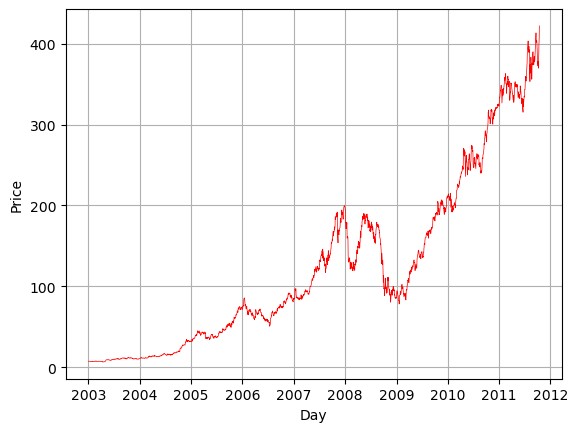
We notice how financial data has lots of ups and downs and if we zoom into the data the change from one day to the next actually tells us very little. This is why we often use rolling functions to understand the data. Here we will calculate a rolling average and plot it with the data.
Here we will calculate a mean over a 250 day window. You have to choose what window to use! As the window slides across the timeseries the data on the right becomes part of the average and the data from the left leaves the average.
rolling_ave = df_resample[my_col].rolling(250).mean()

plt.plot(df_resample.index,df_resample[my_col],'r-',linewidth=.5,label='Data')
plt.plot(df_resample.index,rolling_ave,'k-',linewidth=.8,label='Rolling Average')
plt.grid()
plt.xlabel('Day')
plt.ylabel('Price')
plt.legend()

plt.show()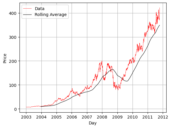
# Do a rolling average of 100 days
rolling_ave = df_resample[my_col].rolling('100D').mean()

plt.plot(df_resample.index,df_resample[my_col],'r-',linewidth=.5,label='Data')
plt.plot(df_resample.index,rolling_ave,'k-',linewidth=.8,label='Rolling Average')
plt.grid()
plt.xlabel('Day')
plt.ylabel('Price')
plt.legend()

plt.show()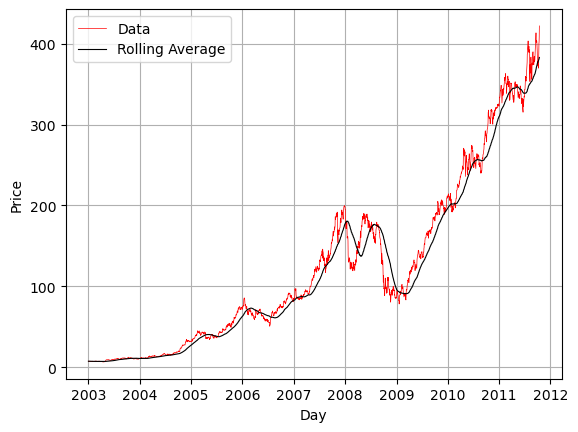
By default .rolling() cannot deal with NaN values. However there is an optional flag `min_periods=’ which lets you specify the minumum number of non-nan values that can be used to calculate. This way NaNs can be dropped.
Sometimes instead of a rolling window, you want an expanding window. For example we could calculate the average as we expand our data over time. In this case the right edge of the window expands to include more data in the average.
expand_ave = df_resample[my_col].expanding().mean()

plt.plot(df_resample.index,df_resample[my_col],'r-',linewidth=.5,label='Data')
plt.plot(df_resample.index,expand_ave,'k-',linewidth=.8,label='Expanding Average')
plt.grid()
plt.xlabel('Day')
plt.ylabel('Price')
plt.legend()

plt.show()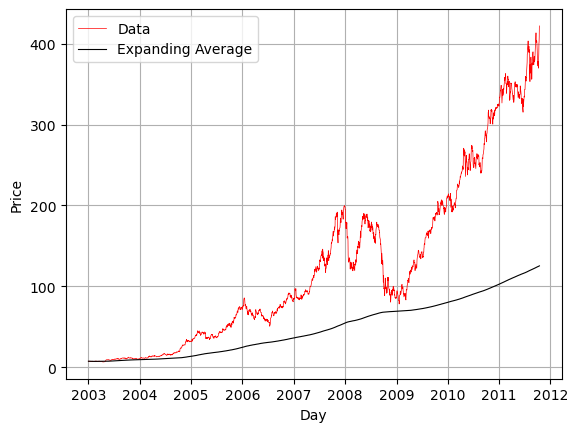
Exponentially Weighted Functions (EWM)
These compute statistics using exponentially decaying weights, giving more importance to more recent data points.
Use cases: - Real-time trend tracking (e.g., financial indicators) - Adaptive smoothing for changing behavior - Faster reaction to recent changes compared to rolling averages
Why it’s useful: - More responsive to recent data - Does not require a fixed window size - Better suited for evolving or rapidly changing data
In Pandas we will use the ewm() exponentially weighted moving function. Here we thing of applying a decay factor based on the span which determines how much memory the ewm has. Often we combine exponential weighting with moving average so that the most recent data has more of an impact on the outcome.
rolling_ave = df_resample[my_col].rolling(250).mean()

# We apply the exponential weighting to the rolling data
# Here we use a span of 30 days.
ewm_rolling_ave = rolling_ave.ewm(span=30).mean()

plt.plot(df_resample.index,df_resample[my_col],'r-',linewidth=.5,label='Data')
plt.plot(df_resample.index,rolling_ave,'k-',linewidth=.8,label='Rolling Average')
plt.plot(df_resample.index,ewm_rolling_ave,'b-',linewidth=.8,label='EWM Rolling Average')
plt.grid()
plt.xlabel('Day')
plt.ylabel('Price')
plt.legend()

plt.show()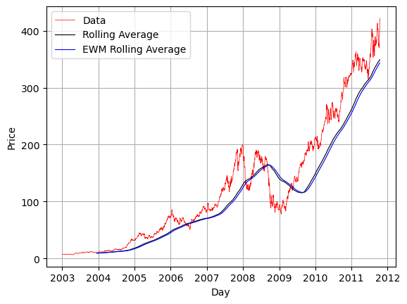
Binary Moving Window Functions
When you are calculating things that need more than one set of timeseries data, for example correlation or covariance, you need to send in additional data into the functions. Here we will plot the correlation between the percent change in the stock price of ‘AAPL’ compared to the percent change in the benchmark index ‘SPX’
# Get the percent changes
pcng_spx = df_resample['SPX'].pct_change()
pcng_aapl = df_resample['AAPL'].pct_change()
# Now calculate the correlation
corr = pcng_aapl.rolling(250).corr(pcng_spx)plt.plot(df_resample.index,corr,'r-',linewidth=.8,label='Correlation Coef')
plt.grid()
plt.xlabel('Day')
plt.ylabel('Correlation')
plt.legend()
plt.ylim([0,1])
plt.show()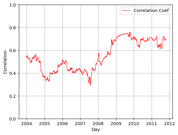
You Try
Add the other two stocks to the correlation graph above. Make sure to label the graph clearly and make it look nice! Experiment with different values for your moving average window. What happens when you change this and why?
# Your code here