import numpy as np
import pandas as pd

import matplotlib.pyplot as plt
import plotly.express as px
from plotly.subplots import make_subplots
import plotly.io as pio
pio.renderers.defaule = 'colab'

from itables import show

# This stops a few warning messages from showing
pd.options.mode.chained_assignment = None
import warnings
warnings.simplefilter(action='ignore', category=FutureWarning)Introduction to Data Science
Data Visualization and Effective Storytelling
Important Information
- Email: joanna_bieri@redlands.edu
- Office Hours: Duke 209 Click Here for Joanna’s Schedule
Announcements
In TWO WEEKS - Data Ethics You should have some resources (book or 3-4 articles) about some area of data science ethics/impacts.
Day 10 Assignment - same drill.
- Make sure Pull any new content from the class repo - then Copy it over into your working diretory.
- Open the file Day3-HW.ipynb and start doing the problems.
- You can do these problems as you follow along with the lecture notes and video.
- Get as far as you can before class.
- Submit what you have so far Commit and Push to Git.
- Take the daily check in quiz on Canvas.
- Come to class with lots of questions!
How to make better Data Visualizations
- Keep it simple!
- Make it easy to see the distinction between categories.
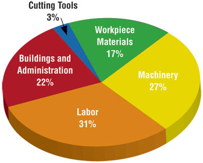
Use color to draw attention
Tell a story - annotate if needed.
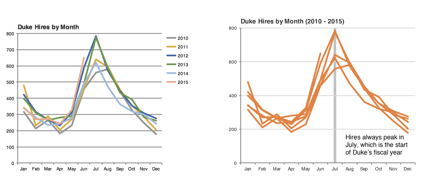
** Pictures thanks to Data Science in a Box.
Principles
- Order Matters
- Put long categories on the y-axis
- Pick a Purpose.
- Keep scales consistent
- Select meaningful colors
- Use meaningful and nonredundant labels.
Let’s work through an example.
Data - September 2019 - YouGov survey asked 1,639 adults in Great Britain:
In hindsight, do you think Britain was right/wrong to vote to leave EU?
They had the choices:
- Right to leave
- Wrong to leave
- Don’t know
Source: YouGov Survey Results, retrieved Oct 7, 2019
This lab follows the Data Science in a Box lectures “Unit 2 - Deck 14: Tips for effective data visualization” by Mine Çetinkaya-Rundel. It has been updated for our class and translated to Python by Joanna Bieri.
Here is the data
file_name = 'data/brexit.csv'
DF = pd.read_csv(file_name)
DF| vote | location | count | |
|---|---|---|---|
| 0 | Right | total | 664 |
| 1 | Wrong | total | 787 |
| 2 | Don’t know | total | 188 |
| 3 | Right | london | 63 |
| 4 | Wrong | london | 110 |
| 5 | Don’t know | london | 24 |
| 6 | Right | rest_of_south | 241 |
| 7 | Wrong | rest_of_south | 257 |
| 8 | Don’t know | rest_of_south | 49 |
| 9 | Right | midlands_wales | 145 |
| 10 | Wrong | midlands_wales | 152 |
| 11 | Don’t know | midlands_wales | 57 |
| 12 | Right | north | 176 |
| 13 | Wrong | north | 176 |
| 14 | Don’t know | north | 48 |
| 15 | Right | scot | 39 |
| 16 | Wrong | scot | 92 |
| 17 | Don’t know | scot | 10 |
Exploring some bar plots
Start with a basic bar plot of all the data!
Basic bar plot - all votes
mask = DF['location'] == 'total'
DF_plot=DF[mask]

fig = px.bar(DF_plot,x='vote',y='count')

fig.show()
Order Matters! Reorder the data by frequency.
Sometimes we want the labels to be alphabetical. We did this in our last class:
yaxis={'categoryorder': 'category descending'}Here are all the possible options for the ‘categoryorder’:
        ['trace', 'category ascending', 'category descending',
        'array', 'total ascending', 'total descending', 'min
        ascending', 'min descending', 'max ascending', 'max
        descending', 'sum ascending', 'sum descending', 'mean
        ascending', 'mean descending', 'median ascending', 'median
        descending']
In this case it seems like we want to have the order ascending by the total amount.
fig = px.bar(DF_plot,x='vote',y='count')

fig.update_layout(xaxis={'categoryorder': 'total descending'},
                  autosize=False,
                  width=800,
                  height=500)

fig.show()
Fix up the figure options
Here I added a bunch of options that we learned from last time.
fig = px.bar(DF_plot,x='vote',y='count',
            color_discrete_sequence=['gray'])

fig.update_layout(xaxis={'categoryorder': 'total descending'},
                  title='Count of Votes in YouGov Survey',
                  xaxis_title="Opinion",
                  yaxis_title="Count",
                  template='ggplot2',
                  autosize=False,
                  width=800,
                  height=500)

fig.show()
Order Matters! Basic Bar Plot - votes by region
First we need to get some data about the votes per region.
DF_plot = DF.groupby('location',as_index=False).sum().copy()DF_plot| location | vote | count | |
|---|---|---|---|
| 0 | london | RightWrongDon’t know | 197 |
| 1 | midlands_wales | RightWrongDon’t know | 354 |
| 2 | north | RightWrongDon’t know | 400 |
| 3 | rest_of_south | RightWrongDon’t know | 547 |
| 4 | scot | RightWrongDon’t know | 141 |
| 5 | total | RightWrongDon’t know | 1639 |
mask = DF_plot['location'] != 'total'
DF_plot = DF_plot[mask]


fig = px.bar(DF_plot,x='location',y='count')
fig.show()
Order Matters! Choose a better order of the categories
Is there an better order here?
In the original survey the order was presented as:
['london','rest_of_south','midlands_wales','north','scot']We can choose a manual ordering using
xaxis={'categoryorder': 'array', 'categoryarray': ['london','rest_of_south','midlands_wales','north','scot']}fig = px.bar(DF_plot,x='location',y='count')
fig.update_layout(xaxis={'categoryorder': 'array', 'categoryarray': ['london','rest_of_south','midlands_wales','north','scot']})
fig.show()Clean up the labels
DF_plot['location']=DF_plot['location'].replace(old category,new_category)DF_plot['location'].replace('london','London',inplace=True)
DF_plot['location'].replace('rest_of_south','Rest of South',inplace=True)
DF_plot['location'].replace('midlands_wales','Midlands and Wales',inplace=True)
DF_plot['location'].replace('north','North',inplace=True)
DF_plot['location'].replace('scot','Scotland',inplace=True)DF_plot| location | vote | count | |
|---|---|---|---|
| 0 | London | RightWrongDon’t know | 197 |
| 1 | Midlands and Wales | RightWrongDon’t know | 354 |
| 2 | North | RightWrongDon’t know | 400 |
| 3 | Rest of South | RightWrongDon’t know | 547 |
| 4 | Scotland | RightWrongDon’t know | 141 |
fig = px.bar(DF_plot,x='location',y='count',color_discrete_sequence=['gray'])
fig.update_layout(xaxis={'categoryorder': 'array', 'categoryarray': ['London','Rest of South','Midlands and Wales','North','Scotland']},
title='Count of Votes in YouGov Survey - Location Level',
xaxis_title="Location",
yaxis_title="Count of Votes",
template='ggplot2',
autosize=False,
width=800,
height=500)
fig.show()Put long labels on y-axis! Flip the bar chart around
- Do this with long labels
- Do this when you have lots of bars
my_categories = ['London','Rest of South','Midlands and Wales','North','Scotland']
fig = px.bar(DF_plot,y='location',x='count',color_discrete_sequence=['gray'])
fig.update_layout(yaxis={'categoryorder': 'array', 'categoryarray': my_categories },
title='Count of Votes in YouGov Survey - Location Level',
xaxis_title="Count of Votes",
yaxis_title="Region",
template='ggplot2',
autosize=False,
width=800,
height=500)
fig.show()Order Still Matters. Reverse the category order
This really depends on your preference. You get to choose the order here.
Here we also removed the y-axis label. Part of making a great plot is to keep it simple but you must Know your audience. If the audience is for people who would know that these are regions then leave the label off. But if the audience might now know these are regions then you should leave the label on.
my_categories.reverse()
fig = px.bar(DF_plot,y='location',x='count',color_discrete_sequence=['gray'])
fig.update_layout(yaxis={'categoryorder': 'array', 'categoryarray': my_categories},
title='Count of Votes in YouGov Survey - Location Level',
xaxis_title="Count of Votes",
yaxis_title="",
template='ggplot2',
autosize=False,
width=800,
height=500)
fig.show()Pick a purpose.
Do opinions about Brexit depend on region?
In the graphs above we did not really answer the question. The graphs above told us about overall number of votes and the number of respondents in each region. But not the breakdown of votes per region.
When making a graph it really helps to have a question to ask. You want to make sure that you are clearly telling a story. You want to draw the eye to the important information. Always ask: Am I clearly answering my question with this picture?
mask = DF['location'] != 'total'
DF_plot=DF[mask]
DF_plot['location'].replace('london','London',inplace=True)
DF_plot['location'].replace('rest_of_south','Rest of South',inplace=True)
DF_plot['location'].replace('midlands_wales','Midlands and Wales',inplace=True)
DF_plot['location'].replace('north','North',inplace=True)
DF_plot['location'].replace('scot','Scotland',inplace=True)my_categories = ['London','Rest of South','Midlands and Wales','North','Scotland']
fig = px.bar(DF_plot,y='location',x='count',
color='vote',
color_discrete_sequence=px.colors.qualitative.Safe)
fig.update_layout(yaxis={'categoryorder': 'array', 'categoryarray': my_categories },
title='Count of Votes in YouGov Survey - Location Level',
xaxis_title="Count of Votes",
yaxis_title="Vote",
template='ggplot2',
autosize=False,
width=800,
height=500)
fig.show()my_categories = ['London','Rest of South','Midlands and Wales','North','Scotland']
fig = px.bar(DF_plot,y='vote',x='count',
color='location',
facet_col='location',
color_discrete_sequence=px.colors.qualitative.Safe)
fig.for_each_annotation(lambda a: a.update(text=a.text.split("=")[1]))
my_categories = ['Dont know','Right','Wrong']
fig.update_layout(yaxis={'categoryorder': 'array', 'categoryarray': my_categories},
title='Count of Votes in YouGov Survey - Location Level',
yaxis_title="",
template='ggplot2',
legend_title='Location',
autosize=False,
width=1000,
height=500)
fig.show()Q Which of the plots do you think is better. What you do notice are the pluses and minuses of each figure?
Q Is there any redundancy in the second graph? What is redundant?
Avoid Redundancy
Here is the same graph again, but avoiding redundancy.
my_categories = ['London','Rest of South','Midlands and Wales','North','Scotland']

fig = px.bar(DF_plot,y='vote',x='count',
             facet_col='location',
            color_discrete_sequence=['gray'])

fig.for_each_annotation(lambda a: a.update(text=a.text.split("=")[1]))

my_categories = ['Dont know','Right','Wrong']
fig.update_layout(yaxis={'categoryorder': 'array', 'categoryarray': my_categories},
                  title='Count of Votes in YouGov Survey - Location Level',
                  yaxis_title="",
                  template='ggplot2',
                  legend_title='Location',
                  autosize=False,
                  width=1000,
                  height=500)

fig.show()
This is a little more boring, since we are avoiding reduncy we are avoiding the old coloring. One way to keep the coloring but to take out some redundancy is to remove the legend.
my_categories = ['London','Rest of South','Midlands and Wales','North','Scotland']

fig = px.bar(DF_plot,y='vote',x='count',
             color='location',
             facet_col='location',
            color_discrete_sequence=px.colors.qualitative.Safe)

fig.for_each_annotation(lambda a: a.update(text=a.text.split("=")[1]))

my_categories = ['Dont know','Right','Wrong']
fig.update_layout(yaxis={'categoryorder': 'array', 'categoryarray': my_categories},
                  title='In hindsight, do you think Britain was right/wrong to vote to leave EU?',
                  yaxis_title="",
                  template='ggplot2',
                  legend_title='Location',
                  autosize=False,
                  width=1000,
                  height=500,
                 showlegend=False)

fig.show()
Q Which of these two plots do you like better and why?
Selecting meaningful colors.
Here is a great website for selecting beautiful colors!
my_categories = ['London','Rest of South','Midlands and Wales','North','Scotland']

fig = px.bar(DF_plot,y='vote',x='count',
             color='vote',
             facet_col='location',
             color_discrete_map={'Right':'#91bfdb','Wrong':'#fc8d59',"Don’t know":'#ffffbf'})

fig.for_each_annotation(lambda a: a.update(text=a.text.split("=")[1]))

my_categories = ['Dont know','Right','Wrong']
fig.update_layout(yaxis={'categoryorder': 'array', 'categoryarray': my_categories},
                  title='In hindsight, do you think Britain was right/wrong to vote to leave EU?',
                  yaxis_title="",
                  template='ggplot2',
                  legend_title='Location',
                  autosize=False,
                  width=1000,
                  height=500,
                 showlegend=False)

fig.show()
Exercise 1 (Choose one!)
Data Vis Principles:
- Order Matters
- Put long categories on the y-axis
- Pick a Purpose.
- Keep scales consistent
- Select meaningful colors
- Use meaningful and nonredundant labels.
Option 1.
Create your own plot of this data. Make it as nice as possible! Choose your own colors, themes, labels, ordering, etc. Decide if you prefer facets or colored bars. Make the labels as informative as possible. Try experimenting with things we haven’t yet covered in class: look up how to add a caption or include textures in your plot.
Talk about the positives and negatives of your graph. How does it meet, not meet, or exceed the data visualization principles above?
Option 2.
Using data of your choice, create a beautiful data visualization. Try experimenting with things we haven’t yet covered in class: look up how to add a caption or include textures in your plot.
Talk about the positives and negatives of your graph. How does it meet, not meet, or exceed the data visualization principles above?