# We will just go ahead and import all the useful packages first.
import numpy as np
import sympy as sp
import pandas as pd
import matplotlib.pyplot as plt

# Special Functions
from sklearn.metrics import r2_score, mean_squared_error

# Functions to deal with dates
import datetimeMath for Data Science
Calculus - Limits
Important Information
- Email: joanna_bieri@redlands.edu
- Office Hours take place in Duke 209 unless otherwise noted – Office Hours Schedule
Today’s Goals:
- Start our discussion of topics in Calculus.
- Taking Limits
Where are we?
So far we have reviewed important concepts to get more comfortable with ideas like:
- Fractions
- Exponents and Logarithms
- Functions and graphing
We applied these ideas to real data using regression:
- We can do feature engineering - apply functions to our data.
- Given data we can fit a curve to it and use it for predictions.
But what more can we do with these curves, functions, ideas?
NOTE - just because we are moving into the study of calculus, does not mean these concepts will go away. Please keep practicing if you need to and never be ashamed of going back and relearning something. I often have to learn things 3-4 times before I really get it and start to remember it!
Calculus is the study of continuous change.
In Data Science we are often interested in how variables change in relation to one another. We know how to find relationships like:
\[ y = \beta_0 + \beta_1 f_1(x) + \beta_2 f_2(x) + \dots \]
but what do we do with this information after we have it? What more can we say about the relationship between \(y\) and \(x\). Here are things calculus can help us with:
- Rates of change or curvature.
- Long term predicted behavior.
- Finding maximums and minimums.
- Developing tools to be used in probability, regression, and machine learning.
Limits
Limits are a mathematical idea that help us understand how a function behaves as we get close to a given point. Limits form the basis for all of calculus! Let’s start with some notation:
\[ \lim_{x\rightarrow a} f(x) \]
This is just a fancy way to write: “What happens to \(f(x)\) as we get really really really close to \(x=a\).”
How would you put the following notation into words?
\[ \lim_{x\rightarrow \infty} e^{-x} \]
.
.
.
.
To me this reads “What happens to the function \(e^{-x}\) as we get really really really close to \(x=\infty\)… knowing that we can’t ever actually reach infinity.
It is a persnickety point, but when we think about limits we don’t ever actually let \(x\) reach the point. We are just thinking about what happens as we get super close to the point from either side.
To find a limit we imagine getting closer to the given point \(a\) from both the left and right side. The answer to a limit can take a few possible options:
- The answer is just a number \(N\), then we say $ _{xa} f(x) = N$.
- The answer just gets more and more positive or more and more negative, never stopping, then we say $ _{xa} f(x) = DNE$ does not exist.
- In some cases the answer fluctuates, but we can’t pinpoint a single number, then we say $ _{xa} f(x) = DNE$ does not exist.
An Example
\[ \lim_{x\rightarrow 2} x^2 \]
You can probably guess what the result is, but we are going to explore this in excruciating detail just for fun!!!
- Look at a graph and imagine walking closer and closer to \(x=2\).
- See what happens as we plug \(x\) values closer and closer to \(x=2\) into our function \(f(x) = x^2\). Notice we could approach \(x=2\) from the right or the left!
x = np.arange(0,4,.01) # Choose the x-values (LEFT,RIGHT,STEP)
def f(x):
    return x**2 # Function
a = 2 # The point we are sending x to


# You should not need to change the code below
y = f(x)
ya = f(a)
plt.plot(x,y,'-b')
plt.grid()
plt.plot(a,ya,'or')
plt.show()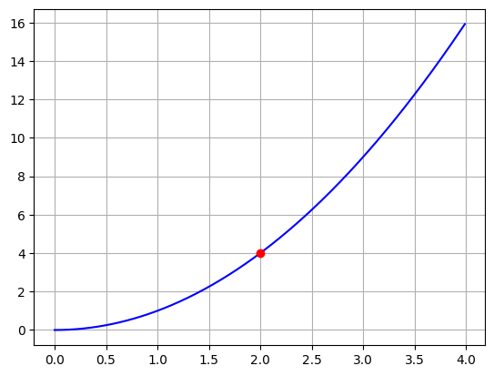
# From the LEFT
x = 0 # Starting Point to the left of a
def f(x):
    return x**2 # Function

# You should not need to change the rest.
dx = 1
LIM = 'yes'
while LIM == 'yes':
    for i in range(10):
        print(f'x={x} and f(x) = {f(x)}')
        x += dx
        dx /=2

    LIM = input('Continue the limit (yes/no):').lower()
x=0 and f(x) = 0
x=1 and f(x) = 1
x=1.5 and f(x) = 2.25
x=1.75 and f(x) = 3.0625
x=1.875 and f(x) = 3.515625
x=1.9375 and f(x) = 3.75390625
x=1.96875 and f(x) = 3.8759765625
x=1.984375 and f(x) = 3.937744140625
x=1.9921875 and f(x) = 3.96881103515625
x=1.99609375 and f(x) = 3.9843902587890625Continue the limit (yes/no): no# From the RIGHT
x = 4 # Starting Point to the right of a
def f(x):
return x**2 # Function
# You should not need to change the rest.
dx = 1
LIM = 'yes'
while LIM == 'yes':
for i in range(10):
print(f'x={x} and f(x) = {f(x)}')
x -= dx
dx /=2
LIM = input('Continue the limit (yes/no):').lower()x=4 and f(x) = 16
x=3 and f(x) = 9
x=2.5 and f(x) = 6.25
x=2.25 and f(x) = 5.0625
x=2.125 and f(x) = 4.515625
x=2.0625 and f(x) = 4.25390625
x=2.03125 and f(x) = 4.1259765625
x=2.015625 and f(x) = 4.062744140625
x=2.0078125 and f(x) = 4.03131103515625
x=2.00390625 and f(x) = 4.0156402587890625Continue the limit (yes/no): noNo matter which way we look at it we see
\[ \lim_{x\rightarrow 2} x^2 = 4 \]
Now I totally remember thinking: WHY NOT JUST PLUG IN \(4\)!?!?!?! Well, this is because there are cases where this would get your in trouble and it is not the mathematically correct interpretation of the limit.
You Try
Redo the analysis above for the following limits:
\[ \lim_{x\rightarrow 2} x^3\]
\[ \lim_{x\rightarrow 1} \ln(x)\]
\[ \lim_{x\rightarrow 0} \frac{1}{x}\]
What happens in this last case? Do you get an error in the code?
Limits at Infinity
Many times we want to know what happens as \(x\) gets really big or really small:
\[ \lim_{x\rightarrow \infty} \frac{1}{x}\]
in these cases we let \(x\) get bigger and bigger, and just approach from one side. Lets explore this one
x = np.arange(1,40,.1) # Choose the x-values (LEFT,RIGHT,STEP)
def f(x):
    return 1/x # Function
# I can't plug in infinity!

# You should not need to change the code below
y = f(x)
ya = f(a)
plt.plot(x,y,'-b')
plt.grid()
plt.show()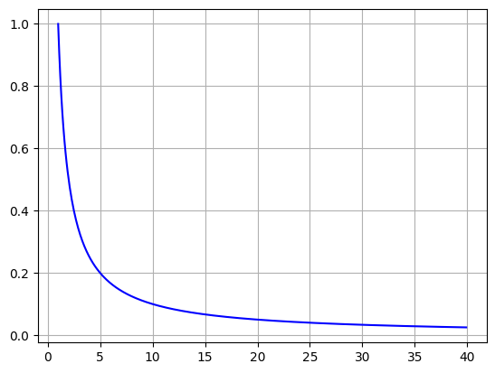
# From the LEFT toward infinity
x = 100 # Starting Point to the left of a
def f(x):
    return 1/x # Function

# You should not need to change the rest.
dx = 1
LIM = 'yes'
while LIM == 'yes':
    for i in range(10):
        print(f'x={x} and f(x) = {f(x)}')
        x += dx
        dx *=2

    LIM = input('Continue the limit (yes/no):').lower()
x=100 and f(x) = 0.01
x=101 and f(x) = 0.009900990099009901
x=103 and f(x) = 0.009708737864077669
x=107 and f(x) = 0.009345794392523364
x=115 and f(x) = 0.008695652173913044
x=131 and f(x) = 0.007633587786259542
x=163 and f(x) = 0.006134969325153374
x=227 and f(x) = 0.004405286343612335
x=355 and f(x) = 0.0028169014084507044
x=611 and f(x) = 0.0016366612111292963Continue the limit (yes/no): noHere we see that as \(x\rightarrow \infty\) our function \(\frac{1}{x}\) gets smaller and smaller toward zero. So we would say:
\[ \lim_{x\rightarrow \infty} \frac{1}{x}=0\]
You Try
Redo the analysis above for the following limits:
\[ \lim_{x\rightarrow \infty} e^{-x}\]
\[ \lim_{x\rightarrow -\infty} x^3\]
\[ \lim_{x\rightarrow \infty} \sin(x)\]
Remember if you can’t get just one single number, then the limit does not exist.
More complicated Limits
We can take limits of more complicated combinations of functions. To do this we need algebra, some properties of limits, and some instincts about functions.
More complicated Limits - Algebra
Sometimes we can just use algebra to simplify our limits:
\[ \lim_{x\rightarrow \infty} \frac{x}{x^2}\]
well this is the same as
\[ \lim_{x\rightarrow \infty} \frac{1}{x}\]
which we solved above!
More complicated Limits - Properties of limits
Assume that \[ \lim_{x \to a} f(x) = L \;\;\;\;\;\;\; \lim_{x \to L} g(x) = M \]
- Sum and Difference Property
\[ \lim_{x \to a} \left[ f(x) \pm g(x) \right] = \lim_{x \to a} f(x) \pm \lim_{x \to a} g(x) = L \pm M. \]
- Product Property:
\[ \lim_{x \to a} \left[ f(x) \cdot g(x) \right] = \lim_{x \to a} f(x) \cdot \lim_{x \to a} g(x) = L \cdot M. \]
- Quotient Property: (provided that $ M $)
\[ \lim_{x \to a} \left[ \frac{f(x)}{g(x)} \right] = \frac{\lim_{x \to a} f(x)}{\lim_{x \to a} g(x)} = \frac{L}{M}. \]
- Constant Multiple Property:
\[ \lim_{x \to a} \left[ c \cdot f(x) \right] = c \cdot \lim_{x \to a} f(x) = c \cdot L, \] where $ c $ is a constant.
Find the limit:
\[ \lim_{x\rightarrow \infty} \frac{x+1}{x^2}\]
use algebra to break it into pieces and then use the sum property:
\[ \lim_{x\rightarrow \infty} \frac{x+1}{x^2} = \lim_{x\rightarrow \infty} \left( \frac{x}{x^2} + \frac{1}{x^2} \right) = \lim_{x\rightarrow \infty} \left( \frac{1}{x} + \frac{1}{x^2} \right)\]
\[= \lim_{x\rightarrow \infty} \frac{1}{x} + \lim_{x\rightarrow \infty}\frac{1}{x^2} = 0+0 = 0\]
You Try
Find the limit:
\[ \lim_{x\rightarrow 3} \frac{x^2+5x}{x+9}\]
More complicated Limits - Instincts about functions.
There are some really interesting special cases:
\[ \lim_{x \to \infty} x^2 e^{-x} \]
well of we use our product property above then we see
\[ \left(\lim_{x \to \infty} x^2\right)\left( \lim_{x \to \infty} e^{-x}\right) = (\infty)(0) = ? \]
for limits like these we have to take into consideration “how fast” or “how dominant” a function is. Lets look at \(y=x^2\) and \(y=e^{-x}\) using a graph and ask the question: Does \(x^2\) reach infinity before \(e^{-x}\) gets to zero?
x  = np.arange(0,5,.1)

def f1(x):
    return x**2

def f2(x):
    return np.exp(-x)

plt.plot(x,f1(x),'-r',label='x^2')
plt.plot(x,f2(x),'-b',label='exp(-x)')
plt.grid()
plt.legend()
plt.show()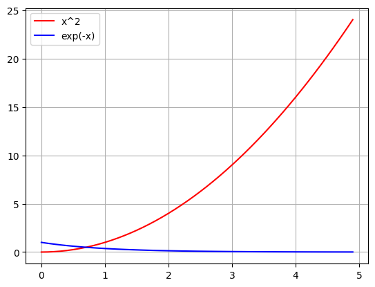
x  = np.arange(0,10,.1)

def f3(x):
    return x**2*np.exp(-x)

plt.plot(x,f3(x),'-k')
plt.grid()
plt.show()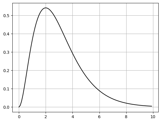
In the graphs above you can see that the decaying exponent function is more powerful! It drags that limit down to zero before \(x^2\) can reach infinity. If we look at the two together, we see that this is what happens. At first the function increases thanks to the \(x^2\) but then it quickly goes to zero. So in this case:
\[ \left(\lim_{x \to \infty} x^2\right)\left( \lim_{x \to \infty} e^{-x}\right) = (\infty)(0) = 0 \]
we can use this kind of instinct to manage problems like:
\[ \lim_{x \to \infty} \frac{x^2 - x + 10}{x^3 + 5x} = \frac{\infty}{\infty} = ? \]
if I think about how quickly the leading functions grow or decay then I can sus out the limit.
x  = np.arange(0,5,.1)

def f1(x):
    return x**2

def f2(x):
    return x**3

plt.plot(x,f1(x),'-r',label='x^2')
plt.plot(x,f2(x),'-b',label='x^3')
plt.grid()
plt.legend()
plt.show()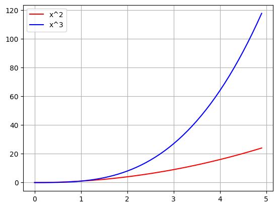
Since the x^3 gets bigger faster, I think it will reach infinity first so this limit should go to zero!
x  = np.arange(.01,5,.1)

def f3(x):
    return (x**2-x+10)/(x**3+5*x)

plt.plot(x,f3(x),'-k')
plt.grid()
plt.show()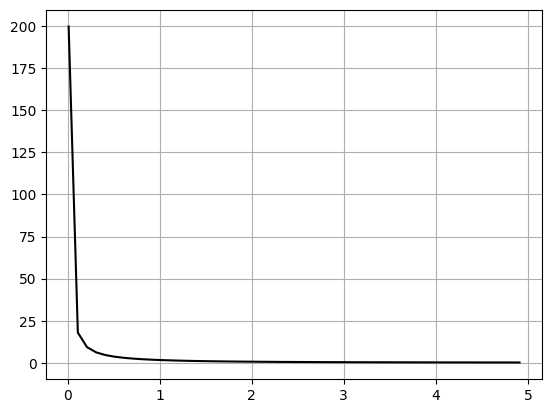
More complicated Limits - Sympy
Sympy has a function sp.limit() that will calculate your limits for you.
\[ \lim_{x \to \infty} \frac{x^2 - x + 10}{x^3 + 5x}\]
# Define the variable
x = sp.symbols('x')
# Define the function:
f = (x**2-x+10)/(x**3+5*x)

# Calculate the limit of f as x approaches a
# limit(f,x,a)
sp.limit(f, x, np.inf)
\(\displaystyle 0\)
so this means
\[ \lim_{x \to \infty} \frac{x^2 - x + 10}{x^3 + 5x} = 0\]
What about this one:
\[ \lim_{x \to \infty} \sin(x) \]
What does the output here mean?
# Define the variable
x = sp.symbols('x')
# Define the function:
f = sp.sin(x)

# Calculate the limit of f as x approaches a
# limit(f,x,a)
sp.limit(f, x, np.inf)
\(\displaystyle \left\langle -1, 1\right\rangle\)
Conclusion
Limits are a way to explore functions and think about what they do as they reach certain points or even go to infinity. What you should be able to do:
- Figure out the limits of our basic functions using either a graph, your instincts, or by plugging in numbers closer and closer to \(x=a\)
- Use algebra, properties of limits, and function instincts to calculate more complicated limits.
- Check your results using Sympy.
You Try
Find the limits. In each case graph the function and talk about what the limit means in that case (aka… I am getting closer and closer to ….). Then figure out the limit using algebra and the properties of the limit. Finally check your answer using Sympy.
- \[ \lim_{x \to 2} \left(x^2 - x + 10\right) \]
- \[ \lim_{x \to 0} \frac{x}{x^3+1} \]
- \[ \lim_{x \to \infty} e^{-x/2} \]
- \[ \lim_{x \to -\infty} \cos(x) \]