Math for Data Science

Calculus - Derivatives

Author

Joanna Bieri
DATA100

Important Information

Email: joanna_bieri@redlands.edu
Office Hours take place in Duke 209 unless otherwise noted – Office Hours Schedule

Today’s Goals:

Turn our understanding of Limits into a definition of the Derivative

# We will just go ahead and import all the useful packages first.
import numpy as np
import sympy as sp
import pandas as pd
import matplotlib.pyplot as plt

# Special Functions 
from sklearn.metrics import r2_score, mean_squared_error

# Functions to deal with dates
import datetime

Limits

Limits are a mathematical idea that help us understand how a function behaves as we get close to a given point.

\[ \lim_{x\rightarrow a} f(x) \]

This is just a fancy way to write: “What happens to $f(x)$ as we get really really really close to $x=a$.”

Derivatives

Derivatives help us capture the idea of rate of change. Here is the notation, assume we have some function $y=f(x)$, then the derivative is written:

\[\frac{dy}{dx} = y'\]

This answers the question: How much does $y$ change as $x$ changes. Sometimes we say “d y by d x$ sometimes we say $y prime$. What would this notation mean:

\[\frac{dT}{dt} = T'\]

If $T$ is temperature and $t$ is time?

This is asking how much does the Temperature change as time moves along -or- what is the rate of change of temperature.

Derivatives - a simple example:

Lets say we have some data that is modeled by a linear fit:

\[y=3x+2\]

where $y$ is commute time in minutes and x is your location in miles away from work. Maybe we want to know something like “How fast is $y$ increasing when $x=2$?” In other words, if I am living $2$ miles from work it takes me $8$ minutes to get to work, how much would my commute change if I moved farther away?

x = np.arange(0,4,.01)
y = 3*x + 2


plt.plot(x,y,'-b')
plt.grid()
plt.plot(2,8,'or')
plt.show()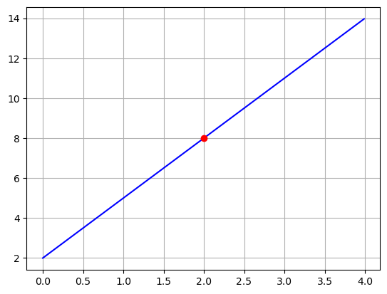

Well, on the graph we can just look at the slope, right? Here since we have the equation we know the slope of the line is $3$.

\[\left. \frac{dy}{dx} \right|_{x=2} = 3\]

So we would say that $y$ changes at a rate of $3$ minutes per mile when $x=2$ and if right now I live $2$ miles away and it takes me $8$ minutes to get to work, then if I move to $3$ miles away my new commute time will be $11$ minutes.

In this simple example the slope does not change as we move around in $x$, so even if I change my question to “How fast is $y$ increasing when $x=3$?”, my answer is the same. I can write down one expression for the rate of change of $y=3x+2$

\[\frac{dy}{dx} = 3\]

What are some things we can say here

The slope of $y$ is $3$
The rate of change of $y$ with respect to $x$ is $3$
$y$ changes at a rate of $3$ minutes per mile.

You Try

Find and interpret the derivative of these lines:

Imagine that $y$ is walking time and $x$ is distance away. \[y=3x+8\] Is it weird that we get the same answer for the rate of change even though we slightly changed our function?

Imagine that $y$ is money in my account in hundreds of dollars and $x$ is the week in the semester. \[y=-x+10\]

Derivatives - a more complicated example:

Now imagine that our data should have been modeled by a polynomial.

\[y=f(x) = 2x^2+2\]

where $y$ is commute time in minutes and x is your location in miles away from work. And now we ask the question “How fast is $y$ increasing when $x=2$?”

x = np.arange(0,4,.01)
y = 2*x**2+2


plt.plot(x,y,'-b')
plt.grid()
plt.plot(2,10,'or')
plt.show()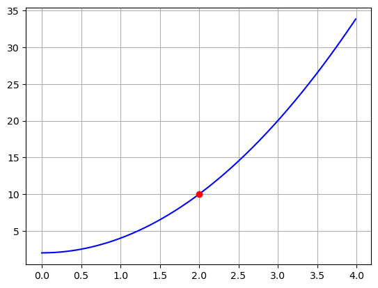

This is a much harder question to answer, because our function is curvy! But lets use what we know about straight lines to try to figure this out.

x = np.arange(0,5,.01)

def f(x):
    return 2*x**2+2
y = f(x)
y_point = 2
dx = 2

# Get the estimated line/slope
x_points = np.array([y_point,y_point+dx])
y_points = f(x_points)
slope = (y_points[1]-y_points[0])/(dx)
y_line = slope*(x-y_point) + f(y_point)

# Graph the results
plt.plot(x,y,'-b')
plt.grid()
plt.plot(x_points,y_points,'or')
plt.plot(x,y_line,'-r')
plt.show()

print(f'The slope of the red line is: {slope}')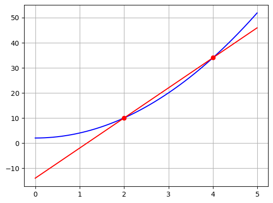

The slope of the red line is: 12.0

First we estimate the slope using the points $(2,10)$ and $(4,34)$

\[slope = \frac{rise}{run}= \frac{f(4)-f(2)}{4-2} = \frac{34-10}{4-2} = \frac{24}{2} = 12\]

The general formula for this can be written with $dx$ is the change in $x$

\[slope = \frac{rise}{run} = \frac{f(2+dx) - f(2)}{dx} \]

Is this an over or under estimate of the actual slope at $x=2$? In other words, is this line steeper or less steep than what the actual answer should be?

This seems too steep to me! How could we do better? We could choose a smaller $dx$:

dx	slope
2	12
1	10
0.5	9
0.25	8.5
0.125	8.25
0.00001	8.000020000054064

So it seems like the best estimate is

\[\left. \frac{dy}{dx} \right|_{x=2} = 8\]

Some things to notice:

As our estimate of the slope at the exact point gets better, the line becomes a tangent line (aka a line that touches the curve at one point but does not cross)
To get the best possible estimate we are SNEAKING UP on $dx=0$… What does this sound like we are doing mathematically?

We are taking a limit!!!

\[slope = \lim_{dx\to 0} \frac{f(2+dx) - f(2)}{dx} = \left. \frac{dy}{dx} \right|_{x=2} \]

What if I change my question to “How fast is $y$ increasing when $x=3$?” Does my answer change?

You Try

Redo the analysis above to solve for

\[ \left. \frac{dy}{dx} \right|_{x=3} \]

Derivatives - of a Function - from limit definition

Wouldn’t it be nice if we didn’t have to redo our analysis every single time we wanted to find the slope of a curve at a point? Well, because we are good at functions and limits we can actually do this!!! Let’s find the general derivative of

\[y=f(x) = 2x^2+2\]

first using the limit and then using sympy! We can write down the definition of the derivative as

\[ \frac{dy}{dx} = \lim_{dx\to 0} \frac{f(x+dx) - f(x)}{dx} \]

So lets plug in our function and do some algebra:

\[ \lim_{dx\to 0} \frac{[2(x+dx)^2+2] - [2x^2+2]}{dx} = \lim_{dx\to 0} \frac{[2(x^2+2xdx+dx^2)+2] - [2x^2+2]}{dx} = \]

\[\lim_{dx\to 0} \frac{[2x^2+4xdx+2dx^2+2] - [2x^2+2]}{dx} = \lim_{dx\to 0} \frac{4xdx+2dx^2}{dx} = \lim_{dx\to 0} 4x+2dx\]

We can take this limit! As $dx $ we see that we are left with $4x$ so we can write

\[ \frac{dy}{dx} = \frac{d}{dx} (2x^2+2) = 4x \]

Now we can just plug in different x-values to find the slope and this matches our analysis above:

\[ \left. \frac{dy}{dx} \right|_{x=2} = 4(2) = 8 \]

\[ \left. \frac{dy}{dx} \right|_{x=3} = 4(3) = 12 \]

Derivatives - of a Function - from Sympy

# Define the function
x = sp.symbols('x')
y = 2*x**2+2

# Take the derivative
sp.diff(y,x)

$\displaystyle 4 x$

You Try

First find the derivative using the limit definition
Then check your answer with sympy

\[y=3x+8\]

\[y=x^3+10\]

Derivatives - what do they tell us?

We already established a few ideas before, but let’s write them down here:

The derivative tells me the slope at a point on a curve.
The derivative tells me the rate of change (instantaneous) at a point on a curve.
The derivative gives me the slope of a tangent line to the curve.

But lets explore a bit more:

\[ y = x^2 \]

Finding the Equation of a tangent line

The general equation for a line is

\[ y = mx + b = (slope)x + (intercept)\]

Well, we have a way to figure out the slope and we can solve for the intercept!

Find the equation of the tangent line to $ y = x^2$ at the point $x=1$:

First calculate the derivative at $x=1$

# Define the function
x = sp.symbols('x')
y = x**2

# Take the derivative
sp.diff(y,x)

$\displaystyle 2 x$

so when $x=1$ the slope is $m=2$ making our line

\[ y = 2x + b\]

Find the value for $b$ that makes the line touch the curve:

This line needs to touch at the point $x=1$ and $f(1) = (1)^2 = 1$ so it goes through the point $(1,1)$. Plug this in ans solve for $b$:

\[ 1 = 2(1) + b \;\;\;\; b = 1-2 = -1\]

Graph to check your results

\[ y = 2x-1\]

and

\[ y = x^2\]

x = np.arange(-2,2,.01)

def f(x):
    return x**2

y = f(x)

tan_line = 2*x-1

plt.plot(x,y,'-b')
plt.plot(x,tan_line,'-r')
plt.grid()
plt.show()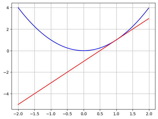

The derivative is the slope of the tangent line!

The cool thing about a tangent line is that you can use it to estimate values of your function near the tangent point. If we look at the graph above we see that the red line is REALLY close to the blue line for values close to $x=1$. So what if I wanted to calculate $f(1.3)$. I could either plug in:

\[(1.3)^2 = 1.6900000000000002 \]

but I could not do this in my head! OR I could plug into the tangent line

\[2(1.3)-1 = 2.6 - 1 = 1.6\]

This is pretty close and I could do the calculation in my head! This is called a linear approximation or linear estimate.

Increasing and Decreasing parts of a function

Here I will plot a few example tangent lines

x = np.arange(-2,2,.01)

def f(x):
    return x**2

y = f(x)

tan_line1 = 2*x-1
tan_line2 = 0*x
tan_line3 = -2*x-1

plt.plot(x,y,'-b')
plt.plot(x,tan_line1,'--r')
plt.plot(x,tan_line2,'--g')
plt.plot(x,tan_line3,'--m')
plt.grid()
plt.show()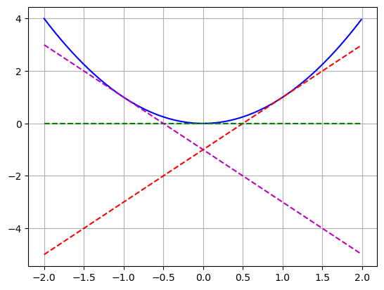

Looking at this graph lets fill in the following conclusions:

If $y$ is decreasing then $\frac{dy}{dx}$, the derivative is ______.
If $y$ is increasing then $\frac{dy}{dx}$, the derivative is ______.
If $y$ is flat then $\frac{dy}{dx}$, the derivative is ______.

Derivatives - Exploring Functions

Now we will consider a more complicated example and see what we can say about a function just from knowing things about its derivative.

\[y = x^3 - x + 1 \]

Calculate the derivative

You should you Sympy… but a great challenge is to try to also do the limit definition!

# Define the function
x = sp.symbols('x')
y = x**3 - x + 1

# Take the derivative
sp.diff(y,x)

$\displaystyle 3 x^{2} - 1$

So the derivative of $y$ is given by

\[y' = 3x^2-1 \]

Plot the function and it’s derivative.

Talk about where the derivative is positive, negative, or zero.

*Here is a plot of my original function $y= x^3 - x + 1$

x = np.arange(-2,2,.01)

def f(x):
    return x**3 - x + 1

y = f(x)

plt.plot(x,y,'-b')
plt.grid()
plt.show()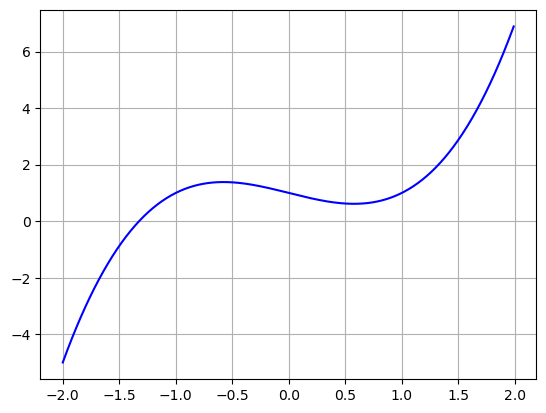

Here is a plot of the derivative $y’ = 3x^2-1 $

x = np.arange(-2,2,.01)

def f_prime(x):
    return 3*x**2 - 1

y_prime = f_prime(x)

plt.plot(x,y_prime,'-r')
plt.grid()
plt.show()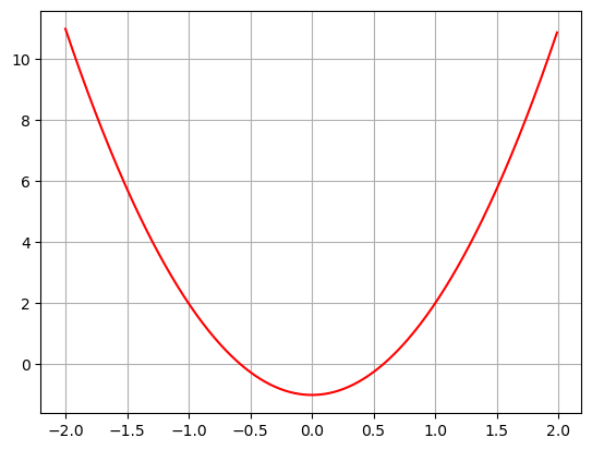

I see that my derivative drops below zero at points between about -0.5 and 0.5. and otherwise it is positive. If I compare back to the plot of my function, is see there is only a small region in the middle where the function seems to be decreasing.

For what values of $x$ is my function increasing? decreasing? Show a graph demonstrating these points.

Well we can use the derivative!

Decreasing

If the derivative is negative then our function is decreasing:

\[3x^2-1 < 0\]

so solving this for $x$ we get

\[ 3x^2 < 1\] \[ x^2 < \frac{1}{3} \] \[ -\frac{1}{\sqrt{3}} < x < \frac{1}{\sqrt{3}} \]

So our function is decreasing between $-\frac{1}{\sqrt{3}}$ and $ $. Confirm these points on our graph:

x = np.arange(-2,2,.01)

def f(x):
    return x**3 - x + 1

y = f(x)

xl = -1/np.sqrt(3)
yl = f(xl)
xr = 1/np.sqrt(3)
yr = f(xr)

plt.plot(x,y,'-b')
plt.plot(xl,yl,'or')
plt.plot(xr,yr,'or')
plt.grid()
plt.show()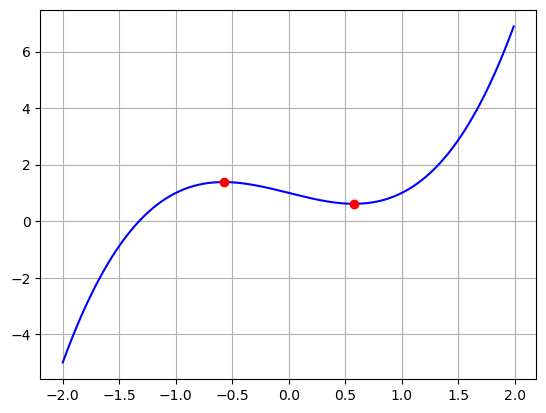

Increasing

If the derivative is positive then our function is increasing:

\[3x^2-1 > 0\]

so solving this for $x$ we get

\[ 3x^2 > 1\] \[ x^2 > \frac{1}{3} \] \[ x<-\frac{1}{\sqrt{3}} \;\;\; or \;\;\; x > \frac{1}{\sqrt{3}} \]

So our function is increasing between $-\frac{1}{\sqrt{3}}$ and $ $. These are the same points on the graph, just on the other side!

What is the rate of change of our function when $x=2$.

For this I can just plug the point $x=2$ into the derivative $y' = 3x^2-1$ so when $x$ is one our rate of change is $y'(2) = 3(2)^2-1 = 11$

Find the equation of a tangent line to the function at the point $x=2$

I already know the slope from the previous question, $m=11$, and I need the line to go through the point $(2,f(2)) = (2,7)$ so I need to solve for $b$

\[ y = 11x+b\] \[ 7 = 11(2) + b\]

so $b=-15$ and my tangent line has the equation $y = 11x-15$. I can plot this to confirm!

x = np.arange(-3,3,.01)

def f(x):
    return x**3 - x + 1

y = f(x)
tan_line = 11*x -15

plt.plot(x,y,'-b')
plt.plot(x,tan_line,'-r')
plt.grid()
plt.show()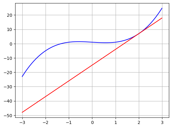

Use the tangent line to estimate the value of our function at $x=2.1$. How close is your estimate?

To do this I plug $x=2.1$ into the tangent line that I found above:

\[ 11(2.1) - 15 = 23.1 - 15 = 8.1 \]

Compare this to the calculated value

2.1**3 - 2.1 + 1

8.161000000000001

So I was correct to the first decimal place.

NOTE how “good” your estimate is has to do with how curvy your function is!

You Try:

Redo the analysis above

Calculate the derivative
Plot the function and it’s derivative.
For what values of $x$ is my function increasing? decreasing?
What is the rate of change of our function when $x=2$.
Find the equation of a tangent line to the function at the point $x=2$
Use the tangent line to estimate the value of our function at $x=2.17$. How close is your estimate?

\[y = x^2 + x + 2\]
\[y = x^4\]
\[y = -5x+7\]