# We will just go ahead and import all the useful packages first.
import numpy as np
import sympy as sp
import pandas as pd
import matplotlib.pyplot as plt

# Special Functions
from sklearn.metrics import r2_score, mean_squared_error

# Functions to deal with dates
import datetimeMath for Data Science
Calculus - Applications of Derivatives
Important Information
- Email: joanna_bieri@redlands.edu
- Office Hours take place in Duke 209 unless otherwise noted – Office Hours Schedule
Today’s Goals:
- Continue working on what the derivative means.
- Apply out understanding of derivatives to data
Derivative Definition
We can write down the definition of the derivative as
\[ \frac{dy}{dx} = \lim_{dx\to 0} \frac{f(x+dx) - f(x)}{dx} \]
Remember the idea - we are trying to figure out the slope of the function at a specific point (instantaneous) so we estimate the slope with lines. Our estimate gets better as our \(dx\) gets smaller, so we take a limit. The derivative is the slope of a tangent line at a point.
Derivatives - of a Function - from Sympy
# Define the function
x = sp.symbols('x')
y = 2*x**2+2

# Take the derivative
sp.diff(y,x)
\(\displaystyle 4 x\)
Can we ALWAYS take a derivative?
No, the limit needs to exist!
Consider the absolute value function. It has a sharp corner at \(x=0\), so if we tried to find
\[ \frac{dy}{dx} = \lim_{dx\to 0} \frac{f(x+dx) - f(x)}{dx} \]
at this location we would get different answers depending on if we were taking the limit from the right or the left (\(dx<0\) vs \(dx>0\))
# Define the function
x = np.arange(-2,2,.01)
y = abs(x)

plt.plot(x,y,'-k')
plt.grid()
plt.show()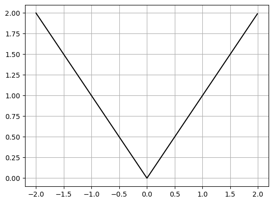
# Define the function
x = sp.symbols('x')
y = abs(x)

# Take the derivative
sp.diff(y,x)
\(\displaystyle \frac{\left(\operatorname{re}{\left(x\right)} \frac{d}{d x} \operatorname{re}{\left(x\right)} + \operatorname{im}{\left(x\right)} \frac{d}{d x} \operatorname{im}{\left(x\right)}\right) \operatorname{sign}{\left(x \right)}}{x}\)
Sympy also struggles to give us an answer for this!
NOTE The derivative is only defined if we can find a tangent line. We can’t find a tangent line at points where there is a sharp corner OR if the slope becomes infinite. In both cases our limit does not exist.
DATA - Applications of Derivative
A slightly contrived practical example
Imagine you have data about the number of visitors to your theme park during most of the days of the year. Here is the data you collected:
y - number of visitors x - day of the year
Lets explore the derivative with this example.
file_location = 'https://joannabieri.com/mathdatascience/data/NationalPark.csv'
DF = pd.read_csv(file_location)
DF.head()| Unnamed: 0 | Visitors | Day | |
|---|---|---|---|
| 0 | 0 | 112.0 | 0 |
| 1 | 1 | 99.0 | 3 |
| 2 | 2 | 113.0 | 6 |
| 3 | 3 | 94.0 | 9 |
| 4 | 4 | 99.0 | 12 |
month_start_days = {
    "January": 0,   # January 1st, 2025 is a Wednesday
    "February": 32, # February 1st, 2025 is a Saturday
    "March": 59,    # March 1st, 2025 is a Saturday
    "April": 90,    # April 1st, 2025 is a Tuesday
    "May": 120,     # May 1st, 2025 is a Thursday
    "June": 151,    # June 1st, 2025 is a Sunday
    "July": 181,    # July 1st, 2025 is a Tuesday
    "August": 212,  # August 1st, 2025 is a Friday
    "September": 243, # September 1st, 2025 is a Monday
    "October": 273, # October 1st, 2025 is a Wednesday
    "November": 304, # November 1st, 2025 is a Saturday
    "December": 334  # December 1st, 2025 is a Monday
}

labels = list(month_start_days.keys())
ticks= list(month_start_days.values())

xreal = DF['Day']
yreal = DF['Visitors']
plt.plot(xreal,yreal,'.k')
plt.grid()
plt.xlabel('Day of Year')
plt.ylabel('Number of Visitors')
plt.xticks(ticks, labels,rotation=45)
plt.show()
plt.show()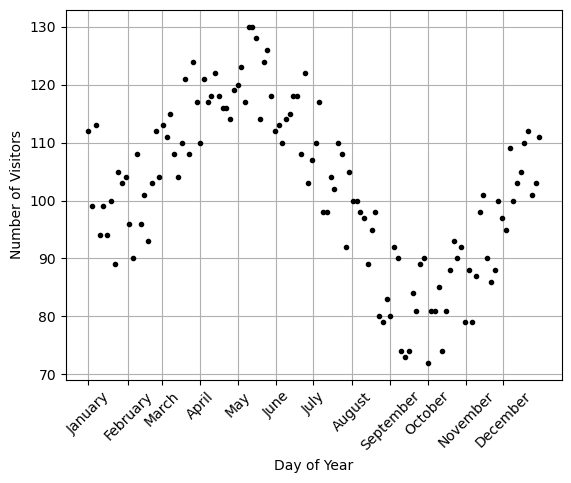
YOU TRY - do a polynomial regression on this data.
# Your code here
Once you have your regression function…
You can enter it in Sympy and ask questions!
This is the function I got from my regression… your answer might be slightly different and that is OKAY!
yfit = -4.80852601194688e-10*xreal**5 +
        4.82804864082977e-7*xreal**4 -
        0.000164214937971268*xreal**3 +
        0.0211869075069019*xreal**2 -
        0.789424620226024*xreal +
        106.945375713063
yfit = -4.80852601194688e-10*xreal**5 + 4.82804864082977e-7*xreal**4 - 0.000164214937971268*xreal**3 + 0.0211869075069019*xreal**2 - 0.789424620226024*xreal + 106.945375713063
plt.plot(xreal,yreal,'k.')
plt.plot(xreal,yfit,'b-')
plt.grid()
plt.xlabel('Day of Year')
plt.ylabel('Number of Visitors')
plt.show()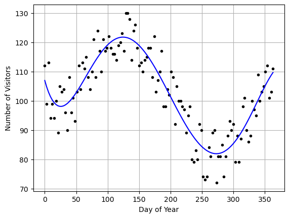
Take the Derivative
# Take the derivative
# Here I reenter the function I got, but now x is a symbol!
x = sp.symbols('x')
y = -4.80852601194688e-10*x**5 + 4.82804864082977e-7*x**4 - 0.000164214937971268*x**3 + 0.0211869075069019*x**2 - 0.789424620226024*x + 106.945375713063

y_p = sp.diff(y,x)
print(y_p)
-2.40426300597344e-9*x**4 + 1.93121945633191e-6*x**3 - 0.000492644813913804*x**2 + 0.0423738150138038*x - 0.789424620226024Plot of the derivative
# Here I copy and paste the derivative and then calculate the y values.
yfit_p = -2.40426300597344e-9*xreal**4 + 1.93121945633191e-6*xreal**3 - 0.000492644813913804*xreal**2 + 0.0423738150138038*xreal - 0.789424620226024
plt.plot(xreal,yfit_p,'m')
plt.grid()
plt.xlabel('Day of Year')
plt.ylabel('Change in the number of Visitors')
plt.show()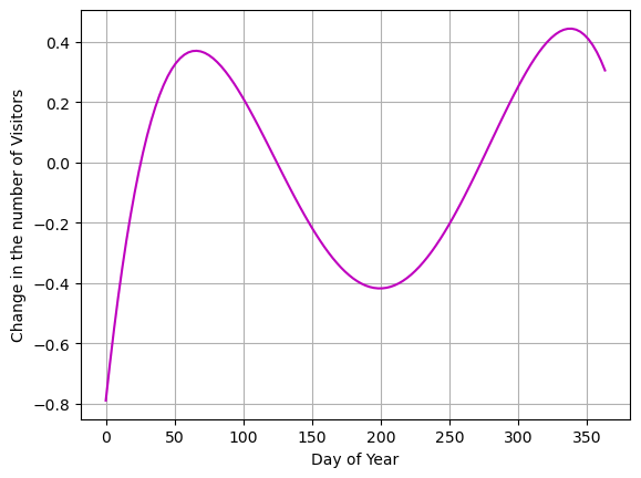
Asking Questions of the Derivative
Now that we have calculated the derivative we can start to ask questions:
- When is my visitation rate decreasing? What day is the rate decreasing the most? What is the rate?
- When is my visitation rate increasing? What day is the rate increasing the most? What is the rate?
- What do these derivatives (rates) mean in terms of my business?
- Can I use the derivative to find which days I had maximum and minimum number of visitors?
- What would the derivative of the derivative tell me?
NEW SYMPY CODE Below I use the sp.roots() this finds the zeros (or roots) of a function
# Decreasing means the derivative is negative.
# Increasing means the derivative is positive.
# Lets find where the derivative is zero.
sp.roots(y_p)
{25.4152067379534: 1,
124.410020212450: 1,
272.889990164400: 1,
380.532785093672: 1}# Plot the derivative and these zeros
plt.plot(xreal,yfit_p,'m')
plt.plot(25.4,0,'or')
plt.plot(124.4,0,'or')
plt.plot(272.9,0,'or')
plt.plot(380.5,0,'or')
plt.grid()
plt.xlabel('Day of Year')
plt.ylabel('Change in the number of Visitors')
plt.show()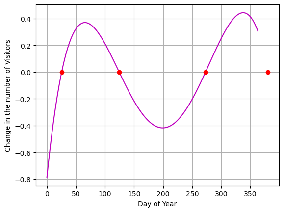
Questions
- Where in this graph is the derivative (change in visitors) negative.
- Where is it positive.
- Where in the graph of the original function (number of visitors) is the derivative negative, positive, zero?
Answers
Here we can see that my visitation is decreasing when: - $ x<25 $ - $ 124<x<273 $
We can see my visitation is increasing when:
- $ 25<x<273$
- $ x>273 $
Because I know this represents a yearly cycle… I might disregard the last number. This is up to my own interpretation using my subject expertise (understanding the data and what it means).
Find the steepest decrease and increase
Using eyeball math:
- It looks like the steepest drop off of visitors is between about 0 and 10
- It looks like the steepest increase in visitors is over between 300 and 365.
How would we actually solve for this?
# We can ask numpy what the maximum derivative value is:
print(f"The max slope is {np.max(yfit_p)}")
# We can find the location of this maximum and look for the associated x-value:
max_loc = np.argmax(yfit_p)
print(f"The max slope is on day {xreal[max_loc]}")
print('----------------')


# Do the same for the minimum
print(f"The min slope is {np.min(yfit_p)}")
min_loc = np.argmin(yfit_p)
print(f"The min slope is on day {xreal[min_loc]}")
The max slope is 0.4442267263190638
The max slope is on day 339
----------------
The min slope is -0.789424620226024
The min slope is on day 0
Lets plot these values on the derivative function
plt.plot(xreal,yfit_p,'m')
plt.plot(339,0.444,'or')
plt.plot(0,-0.789,'ob')
plt.grid()
plt.xlabel('Day of Year')
plt.ylabel('Change in the number of Visitors')
plt.show()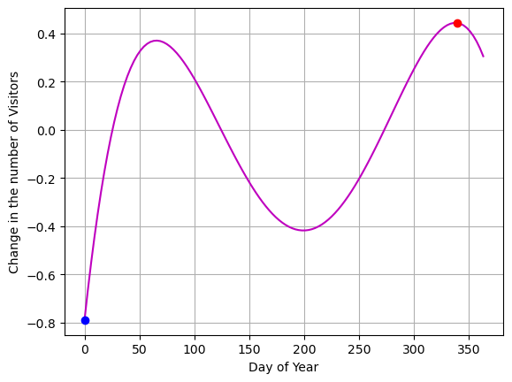
Lets plot these values on the original function
We know the max happens when \(x=339\) and the min happens when \(x=0\) we need to solve for the y_fit values
y1 = y.subs(x,0)
y1
\(\displaystyle 106.945375713063\)
y2 = y.subs(x,339)
y2
\(\displaystyle 100.120697950594\)
plt.plot(xreal,yfit)
plt.plot(339,y2,'or')
plt.plot(0,y1,'ob')
plt.grid()
plt.xlabel('Day of Year')
plt.ylabel('Number of Visitors')
plt.show()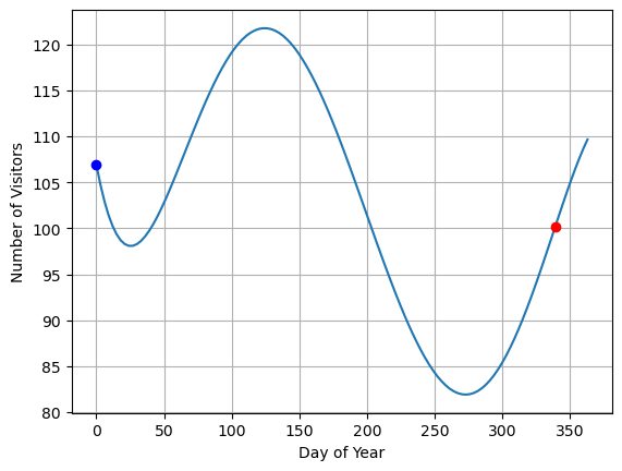
Interpreting the Derivative.
In terms of my business what does all of this mean?
Well if I know that my visitors start decreasing after the first of the year and don’t start rebounding until day 25 (about the end of January), maybe this is a time that I should be doing small maintenance, knowing that visitation is about to start increasing again. I also might need to be careful about scheduling workers. Maybe on day 1 my business feels really over crowded and I am tempted to hire a few new people… but I know this is probably temporary and I should wait to see if I get the expected decrease.
After day 25 we start to see an increase in visitors. I should track my number of employees and plan for the fact we will keep having increasing traffic until around day 124 (about the end of May). After that visitation decreases for quite a while, until day 273 (or about October). During this time frame, if it seems like things are not too busy after the rush, I should transition to maintenance and planning for the next season.
Finally right at the end of the season after day 273 (after October) I should start to see visitation increase for the Holiday rush.
When are my max and min visitation days?
Can the derivative help me answer this question? Better than the data?
Yes the derivative can help me answer this question! Better than the data is hard to say. We could just look through the data and see where the max is, but the data has some noise, so maybe that max will be noisy from year to year?
What happens to the derivative at the functions max/min points?
plt.plot(xreal,yreal,'k.')
plt.plot(xreal,yfit,'b-')
plt.grid()
plt.xlabel('Day of Year')
plt.ylabel('Number of Visitors')
plt.show()
Questions:
- What is the value of the derivative at a max or min point?
- How many max/min points would our derivative find in this case?
- Are all max/min points created equal? In other words, In this picture is on min smaller than another?
- How could the derivative tell us if it is a max or a min?
First Derivative Test
- The function has a local maximum or minimum whenever the derivative equals zero:
\[\frac{dy}{dx}=0\]
we solve this for all of the x-values where this is true, \(x^*\).
- The points \((x^*,y(x^*))\) where the derivative equations zero are called “stationary points” or “critical points”
- We can tell if a critical point is a local max by the derivative going from increasing to decreasing, positive to negative, as we cross the point.
- We can tell if a critical point is a local min by the derivative going from decreasing to increasing, negative to positive, as we cross the point.
We already solved for the zeros before:
# Lets find where the derivative is zero.
sp.roots(y_p)
{25.4152067379534: 1,
124.410020212450: 1,
272.889990164400: 1,
380.532785093672: 1}We will consider each of the critical \(x*\) values that are within our 365 days:
\(x1 = 25.4152067379534\)
\(x2 = 124.410020212450\)
\(x3 = 272.889990164400\)
Look at the slope to the left and to the right of each of these points.
# Start with x1
x1 = 25.4152067379534
xL = x1-1
xR = x1+1

print(y_p.subs(x,xL))
print(y_p.subs(x,xR))
-0.0212733154905305
0.0205638791985034The derivative goes from negative to positive so this must be a local minimum!
y.subs(x,x1)\(\displaystyle 98.0678073386895\)
We have a local minimum at \((25.4,98.1)\)
Our lowest winter visitor numbers happen near the end of January and we can expect around 100 visitors.
YOU TRY
Redo the analysis and interpretation of results for x2 and x3$
Global Maximum and Minimum
So far we have been using the term local max or min. But what we found above is that we have two minimums in our range \([0,365]\). Global maximum and minimum values are the larges over the whole range. In this case we have a global max at about \(x=124\) and a global min at about \(x=273\).
- What if I extended my range \([-\infty,\infty]\)?
- Would these still be global max and min?
YOU TRY
Think about the limit of yfit as \(x\to\pm\infty\)
HINT think about what \(-x^5\) does and look at the plot of our function.
sp.plot(y,(x, 0, 365))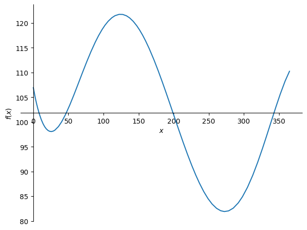
YOU TRY - HOMEWORK 4
Here is some fake data about TV sales in the USA over the course of the year. Imagine this represents TV sales for a large Box store and that you are managing their ordering and number of employees in their TV department.
- Stored in the variable xreal_tv is the day of the year.
- Stored in the variable yreal_tv is the TV sales reported for that day (number of TVs).
- The data is plotted below.
# Just run this to load the data
file_location = 'https://joannabieri.com/mathdatascience/data/tv_sales_data.csv'
DF = pd.read_csv(file_location)
xreal_tv = np.array([i for i in range(len(DF['Date']))])
yreal_tv = DF['TV_Sales']plt.plot(xreal_tv,yreal_tv,'.k')
plt.grid()
plt.xlabel('Date')
plt.ylabel('USA TV Sales')
plt.show()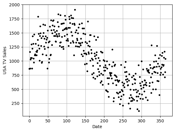
You should do an analysis similar to what we did during this class:
Find a polynomial (or other function if you want a challenge) fit for this data.
Talk about why this is a reasonable fit (correlation, mse, r^2, etc) and where/how it might fail.
Enter your fit function into SYMPY and then take the derivative.
Plot both your fit function and its derivative - explain how you can see on the derivative plot where the fit function is increasing or decreasing.
Use the derivative function to answer the following questions:
- When are TV sales increasing or decreasing?
- When are they increasing or decreasing the most?
- When do sales reach their max or min?
- What are the maximum or minimum sales values?