Math for Data Science

Exam 2 Review

Author

Joanna Bieri
DATA100

Important Information

Email: joanna_bieri@redlands.edu
Office Hours take place in Duke 209 unless otherwise noted – Office Hours Schedule

Today’s Goals:

Review for the exam

About the exam:

My plan is for the exam to be 1 question - yes with multiple parts - but this should be a short more quiz like exam.
Below you will find practice problems. There are WAY more problems to practice than there will be on the exam
During the exam you can have access to your notes and any in-class notebooks that we ran.
The exam will be in the format of an Jupyter Notebook which you can do on Colab (If you have turned off AI assist) or on Jupyter. You can also do some work by hand if you choose.
Code examples will be given for each problem.
If you run into Python errors during the exam, I will be happy to help you debug.
THE MOST IMPORTANT THING is your understanding of what the calculations are doing or what the results mean. Make sure you show all your work. Respond to all the questions in the prompt. Really try to show off your understanding!!

What have we done so far:

We are building on the ideas from the past exam. You should be able to:
- Use Sympy, Numpy, and matplotlib
- Enter functions in symbolic form and do operations with them (sovle, roots, subs)
- Enter functions in numerical form and create a plot of the data
- Use np.polyfit to find a function that fits the data.
New ideas:
- Taking the limit of the function and explaining what the limit tells us. (sp.limit())
- Finding the derivative (or second derivative) of a function (using python) and explaining what the derivative tells us. (sp.diff())
- Using the derivative to find critical points in a function and explaining what they mean.
- Using the first and second derivative tests to optimize - find maximums and minimums. (sp.subs())
- Discuss the difference between a local and global minimum and apply this understanding to your critical points.
- Find critical points of a function of two variables and classify them as max or min.

# We will just go ahead and import all the useful packages first.
import numpy as np
import sympy as sp
import pandas as pd
import matplotlib.pyplot as plt

# Special Functions 
from sklearn.metrics import r2_score, mean_squared_error
from scipy.optimize import curve_fit

Example Code for the exam

# Plotting Numerical Data and Polyfit

# Make up some numerical data
xfake = np.arange(0,5,.05)
noise = np.random.rand(len(xfake))
yfake = 10*xfake**2 + 100*noise

# Find a curve of best fit
betas = np.polyfit(xfake,yfake,2)
yfit = betas[0]*xfake**2+betas[1]*xfake+betas[2]

# Plot the data and the fit
plt.plot(xfake,yfake,'.k')
plt.plot(xfake,yfit,'-r')
plt.grid()
plt.xlabel('x values')
plt.ylabel('y values')
plt.show()

# Print the betas
print(betas)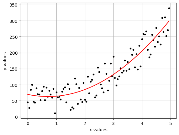

[ 13.12971367 -18.68364267  69.89384863]

# Create a symbolic version of my fit
# Here I switch from xfake to x.
x = sp.symbols('x')
y = betas[0]*x**2+betas[1]*x+betas[2]
y

\(\displaystyle 13.1297136670058 x^{2} - 18.6836426727635 x + 69.8938486252154\)

# Take derivatives
y_p = sp.diff(y,x)
y_pp = sp.diff(y,x,x)

print(y_p)
print(y_pp)

26.2594273340116*x - 18.6836426727635
26.2594273340116

# Solve y_p = 0 for x
sp.solve(y_p,x)

[0.711502289639202]

# Sub a point into a function
y.subs(x,0.421396950750957)

\(\displaystyle 64.3521326003412\)

Data

Below you will load some data for a new business. The data tracks the day number since a new product was released and the number of purchases of that product. The business now wants to study the roll-out of their new items to see if they can improve future roll-outs in the first 100 days of a product launch.

The Question: use what we have learned in data science to analyze this data:

Plot the data.
Create a polynomial fit for the data.
Explain to the business owners why this polynomial fit is the best predictor of these roll-out sales.

Enter the function you found symbolically into python.
Find the derivative of this function.
Use the derivative and test to find and classify critical points in the first 100 days.
Talk about global max/min in the first 100 days.
Explain to the business owners what these derivatives and critical points tell them in terms of their sales. See how much you can say… are there points of very step change? are there days when there is a lot of turn around? what are the sales numbers during the local maxes and mins? what days should they start to look out for decreases in sales, etc.

file_location = 'https://joannabieri.com/mathdatascience/data/mybusiness.csv'
DF = pd.read_csv(file_location)

DF

	Days	Purchases
0	0	290
1	1	280
2	2	810
3	3	590
4	4	790
...	...	...
96	96	1530
97	97	1900
98	98	2100
99	99	1990
100	100	1970

101 rows × 2 columns

# Here is the data
xdata = np.array(DF['Days'])
ydata = np.array(DF['Purchases'])

N=5
betas = np.polyfit(xdata,ydata,N)
yfit = 0
for n,beta in enumerate(betas):
    yfit += beta*xdata**(N-n)

plt.plot(xdata,ydata,'.k')
plt.plot(xdata,yfit,'-r')
plt.grid()
plt.show()

print(f'R^2 value: {r2_score(ydata,yfit)}')
print(f'MSE value: {mean_squared_error(ydata,yfit)}')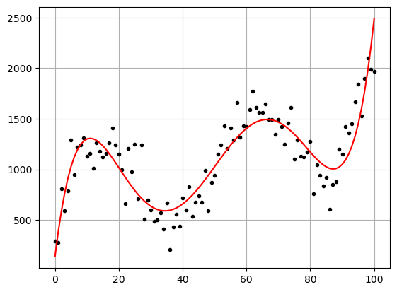

R^2 value: 0.7833537266065624
MSE value: 37134.662149586395

Here I chose to do a polynomial fit using a degree 5 polynomial. In general I would prefer a lower order, simpler, model. But the lower order polynomials did not represent the data well. The degree 5 polynomial has a 0.78 R^2 value, which means that almost 80% of the variance in the data is captured by the model. This is pretty good. It would be hard to get significantly better because the data has quite a bit of noise.

The areas where this fit concerns me the most is at the day 100 end. I wonder if it could be too steep here. Possible gathering more data, or data for more days, would allow us to find a better fit for a long term analysis. As it stands we can only comment on what happens within the 0 to 100 day range.

# Symbolic Representation
x = sp.symbols('x')
y = 0

for n,beta in enumerate(betas):
    y += beta*x**(5-n)

y

\(\displaystyle 2.35481051371161 \cdot 10^{-5} x^{5} - 0.00586184098650973 x^{4} + 0.516663101150162 x^{3} - 18.9546965428993 x^{2} + 259.318996997922 x + 142.890955847142\)

# First derivative
y_p = sp.diff(y,x)
y_p

\(\displaystyle 0.00011774052568558 x^{4} - 0.0234473639460389 x^{3} + 1.54998930345049 x^{2} - 37.9093930857986 x + 259.318996997922\)

# Second derivative
y_pp = sp.diff(y,x,x)
y_pp

\(\displaystyle 0.000470962102742321 x^{3} - 0.0703420918381168 x^{2} + 3.09997860690097 x - 37.9093930857986\)

# Critical points
cps = list(sp.roots(y_p,x))
cps

[11.0325537360738, 34.4380766314611, 66.4909989050391, 87.1827503665473]

# Check each critical point individually
for c in cps:
    print('######################')
    print(f'Testing x*={c}')
    print(f'y(x*)={y.subs(x,c)}')
    print('######################')
    print('---------------------')
    print('First Derivative Test')
    xl = c-1
    xr = c+1
    print(f'Plugging in points to the left: {xl} and the right: {xr} of the critical point: {c}')
    diff_xl = y_p.subs(x,xl)
    diff_xr = y_p.subs(x,xr)
    print(f'Derivative at xl={diff_xl}\nDerivative at xr={diff_xr}')
    if diff_xl<0 and diff_xr>0:
        print(f'This means x*={c} is a MINIMUM')
    elif diff_xl>0 and diff_xr<0:
        print(f'This means x*={c} is a MAXIMUM')
    else:
        print('The first derivative test is inconclusive')
    print('---------------------')
    print('Second Derivative Test')
    print(f'Plugging the critical point x*={x} into the second derivative')
    second_diff_c = y_pp.subs(x,c)
    if second_diff_c > 0:
        print(f'This means x*={c} is a MINIMUM')
    elif second_diff_c < 0:
        print(f'This means x*={c} is a MAXIMUM')
    else:
        print('The second derivative test is inconclusive')
    print('\n')

######################
Testing x*=11.0325537360738
y(x*)=1307.53563738208
######################
---------------------
First Derivative Test
Plugging in points to the left: 10.0325537360738 and the right: 12.0325537360738 of the critical point: 11.0325537360738
Derivative at xl=12.5164174252889
Derivative at xr=-10.7963365289489
This means x*=11.0325537360738 is a MAXIMUM
---------------------
Second Derivative Test
Plugging the critical point x*=x into the second derivative
This means x*=11.0325537360738 is a MAXIMUM


######################
Testing x*=34.4380766314611
y(x*)=591.115224268899
######################
---------------------
First Derivative Test
Plugging in points to the left: 33.4380766314611 and the right: 35.4380766314611 of the critical point: 34.4380766314611
Derivative at xl=-4.68625964721741
Derivative at xr=4.61723752608737
This means x*=34.4380766314611 is a MINIMUM
---------------------
Second Derivative Test
Plugging the critical point x*=x into the second derivative
This means x*=34.4380766314611 is a MINIMUM


######################
Testing x*=66.4909989050391
y(x*)=1493.55727365630
######################
---------------------
First Derivative Test
Plugging in points to the left: 65.4909989050391 and the right: 67.4909989050391 of the critical point: 66.4909989050391
Derivative at xl=4.31905072119116
Derivative at xr=-4.32662337565216
This means x*=66.4909989050391 is a MAXIMUM
---------------------
Second Derivative Test
Plugging the critical point x*=x into the second derivative
This means x*=66.4909989050391 is a MAXIMUM


######################
Testing x*=87.1827503665473
y(x*)=1004.79914614389
######################
---------------------
First Derivative Test
Plugging in points to the left: 86.1827503665473 and the right: 88.1827503665473 of the critical point: 87.1827503665473
Derivative at xl=-9.01583781056161
Derivative at xr=10.5899292420490
This means x*=87.1827503665473 is a MINIMUM
---------------------
Second Derivative Test
Plugging the critical point x*=x into the second derivative
This means x*=87.1827503665473 is a MINIMUM

# Check the endpoints
xright = 0
xleft = 100

print(f'At the right end y(0)={y.subs(x,xright)}')
print(f'At the left end y(100)={y.subs(x,xleft)}')

At the right end y(0)=142.890955847142
At the left end y(100)=2487.87909699618

Okay there is a lot to unpack here:

There are two minimums and two maximums locally in the data.

On about days 34 and 87 we see local minimums in the data. On these days your predicted sales are about 591 and 1005 respectively. These are the biggest slumps in sales, but not the global minimum on the data. The global minimum is at day 0, when you are just rolling out the product and sell about 143 items. This makes sense because overall your sales are increasing even if they hit some local minimums along the way.

On about days 11 and 66 we see local maximums in the data. The predicted sales for these days are about 1308 and 1494 respectively. These are the biggest bumps in your sales over the first 100 days, but we see that the trend is moving upward as we go to days 100 and beyond. On day 100 we see a global max, when you sell about 2488 items.

Lets look at some plots of the derivative function to see where you are seeing the largest increases and decreases in sales.

print(y_p)

0.00011774052568558*x**4 - 0.0234473639460389*x**3 + 1.54998930345049*x**2 - 37.9093930857986*x + 259.318996997922

ydata_p = 0.00011774052568558*xdata**4 - 0.0234473639460389*xdata**3 + 1.54998930345049*xdata**2 - 37.9093930857986*xdata + 259.318996997922

plt.plot(xdata,ydata_p,'-g')
plt.grid()
plt.title('Change in sales over first 100 days')
plt.xlabel('Days')
plt.ylabel('Rate of change of sales')
plt.show()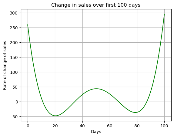

We see that the biggest increases and decreases are at the beginning and end of the time frame. This might mean that you do a good job of advertising your product in the first 11 days, but then something about your roll-out starts to be less effective. After about day 87 it seems that sales are taking off and the as the rate of change increases.

There are two ranges where we see a negative rate of change of sales, aka sales are decreasing. Between days 11 and 34 there are decreases in sales and again between days 66 and 87 there are decreases in sales.

print(y_pp)

0.000470962102742321*x**3 - 0.0703420918381168*x**2 + 3.09997860690097*x - 37.9093930857986

ydata_pp = 0.000470962102742321*xdata**3 - 0.0703420918381168*xdata**2 + 3.09997860690097*xdata - 37.9093930857986

plt.plot(xdata,ydata_pp,'-m')
plt.grid()
plt.title('Change in sales rate over first 100 days')
plt.xlabel('Days')
plt.ylabel('Acceleration of sales')
plt.show()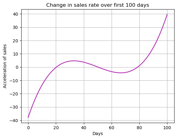

The highest curvature is also at the ends of the data. Your sales start of with a large positive rate of change but loose acceleration quickly. You should try to keep up the momentum from your initial launch. Again toward the end it seems that you have achieved a following for your product and we see the sales accelerate quickly.