# We will just go ahead and import all the useful packages first.
import numpy as np
import sympy as sp
import pandas as pd
import matplotlib.pyplot as plt
from mpl_toolkits.mplot3d import Axes3D

# Special Functions
from sklearn.metrics import r2_score, mean_squared_error

# Functions to deal with dates
import datetimeMath for Data Science
Calculus - Integrals
Important Information
- Email: joanna_bieri@redlands.edu
- Office Hours take place in Duke 209 unless otherwise noted – Office Hours Schedule
Today’s Goals:
- Define the integral
- Understand what the integral means
- How is integration used in Data Science
(Review) Derivative
\[ \frac{dy}{dx} = \lim_{dx\to 0} \frac{f(x+dx) - f(x)}{dx} \]
The derivative gives us information about the slope of the function (or the slope of a tangent line at a point) and they can be used to find critical points and classify critical points as maximums or minimums. This is especially important in optimization.
In Data Science we most often use optimization when building models. We see a model that minimizes a cost function, for example in linear regression we solve for the betas that minimize the square error. This idea of using the slope of a cost function to find a minimum is a basis for all of machine learning.
Integrals - the big idea
I am going to introduce you to the idea of integrals today. We will not use perfect mathematical definitions everywhere here, my goal is that you understand what the integral means and get the feel for how the integral is defined. If you want to really be able to do integrals, you should take MATH 122 (calculus II).
Integrals are the opposite of the derivative. Here is some notation:
\[f(x) = \int F(x) \; dx \]
the s shaped symbol \(\int\) tells us to take the integral, the function \(F(x)\) is called the integrand, and we are integrating with respect to the variable \(x\) based on the fact that we see \(dx\) at the end of the integral.
Because the integral is the opposite of the derivative, in the expression above:
\[\frac{df}{dx} = F(x)\]
Example - integral and derivative
Lets say I have a function and I take the derivative
def f(x):
    return x**3

x = sp.symbols('x')
y = f(x)
y_p = sp.diff(y,x)
y_p
\(\displaystyle 3 x^{2}\)
but then I wanted to “untake” or “undo” the derivative. I could use the integral to do that
# My integrand is the derivative
F = y_p
# This is how I can use sympy to integrate with respect to x
sp.integrate(F,x)
\(\displaystyle x^{3}\)
What this means is that
\[\frac{d}{dx} x^3 = 3x^2\]
AND
\[ \int 3x^2 dx = x^3 \]
so if I know something about the rate of change of a variable I can use the integral to go backward to know about he original variable
Applied Example
Let’s say I know the growth rate of some bacteria - maybe I got a bunch of data and modeled the growth rate over time.
\[ G(t) = 3(t-12)^2-10 \]
Now I want to use this information to predict the amount of bacteria in a sample at time \(t\). Well I want to go from a function that represents growth (number of cells/hour) to a function that just tells me amount (number of cells). This is opposite of rate of change, this is undoing the rate of change. This is exactly what the integral does!
def integrand(t):
return 3*(t-12)**2-10
t = sp.symbols('t')
G = integrand(t)
B = sp.integrate(G,t)
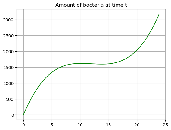
B\(\displaystyle t^{3} - 36 t^{2} + 422 t\)
Lets plot these two functions!
# Get numerical data
tdata = np.arange(0,24,0.1)
Gdata = 3*(tdata-12)**2-10
Bdata= tdata**3 - 36*tdata**2 + 422*tdata # this is G after we integrated

plt.plot(tdata,Gdata,'-r')
plt.title('Growth rate of bacteria at time t')
plt.grid()
plt.show()

plt.plot(tdata,Bdata,'-g')
plt.title('Amount of bacteria at time t')
plt.grid()
plt.show()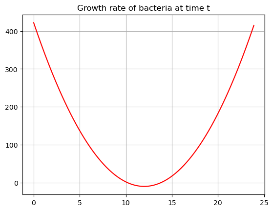
Interpret these results
The growth rate function (red) shows how fast the bacteria is growing at time \(t\). The bacteria is mostly increasing, except for just a little time in the middle of the day where the derivative is negative. There are two critical points where we have no growth.
The bacteria function (blue) which we found by integrating the growth function shows how much bacteria is in the system a time \(t\). We can say exactly how much bacteria we expect to find at time \(t\). We see the function is mostly increasing except for a small range where it slows down.
INTERESTING RELATIONSHIP BETWEEN GRAPHS It turns out that there is a really interesting relationship between these two graphs! We can see the integral visually on the graph…. let’s explore.
Integrals - building up the definition
Let’s think for a minute about how we might go between a function that tells me the rate of change and a function that tells me a value. We will build up this idea using some examples.
Example 1 - Constant Rate of Change
What if we knew that something had a constant rate of change:
\[G(t) = 3\]
bacteria is always growing at a rate of 3 cells per hour. Plot this growth rate:
def growth(t):
    return np.ones(len(t))*3

tdata = np.arange(0,24,0.1)
G = growth(tdata)

plt.plot(tdata,G,'-r')
plt.title('Growth rate of bacteria at time t')
plt.ylim(0,3.5)
plt.grid()
plt.show()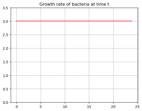
Now ask a question
If I knew that at time \(t=0\) I had exactly \(5\) cells, how many cells would I have when \(t=10\)? How would I calculate this? Just using algebra and instincts:
- The rate of change is \(3\) cells per hour. Every hour we get \(3\) more cells.
- \(t=10\) represents \(10\) hours of time elapsing.
- So, my cells would increase by \(3\times 10 = 30\) cells in \(10\) hours.
- If I started with \(5\) cells then at hour \(10\) I would have \(35\) cells.
But think about this on the graph. What does this multiplication \(3\times 10\) look like?
Its filling in the area under the curve! The total amount of bacteria over that time period is just the area under the curve - BASE times HEIGHT!
start=0
end=10
tfill = np.arange(start,end,0.1)
yfill = growth(tfill)


plt.plot(tdata,G,'-r')
plt.fill_between(tfill, yfill, color='lightblue', alpha=0.7)
plt.title('Growth rate of bacteria at time t')
plt.ylim(0,3.5)
plt.grid()
plt.show()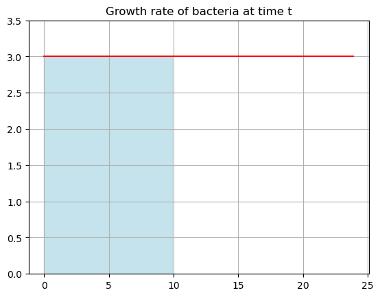
Compare this to the integral.
If I integrate to get the solution to this problem, I find:
\[B(t) = \int 3 \; dt = 3t+c\]
Here I added \(c\) the constant of integration… just knowing the rate of change is not enough, I need to know where I started to know how much I have. So the amount of bacteria at time \(t\) is a straight line function. Look at a graph:
# Consider a whole bunch of starting values
cvals = [0,5,10,15,20]
tdata = np.arange(0,24,0.1)

def bacteria(t,c):
    return 3*t+c

for c in cvals:
    B = bacteria(tdata,c)
    plt.plot(tdata,B,label=f'c={c}')

plt.grid()
plt.title('Ammount of bacteria for different starting values c')
plt.legend()
plt.show()
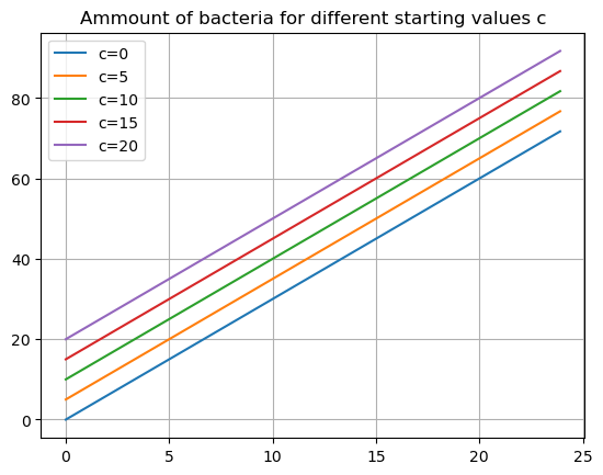
Does this make sense?
- If i started with no bacteria but somehow it was growing at 3 per hour, at hour ten I would have 30 cells.
- If I started with 5, at hour ten I would have 35 cells.
- and so on.
Integration - what do we know
- The integral of a function is related to the area under the curve.
- The solution to the integral is a family of functions where the \(+c\) represents the starting value.
- The integral is the opposite of the derivative.
But we didn’t need calculus for this problem!
Example 2 - Non-Constant Rate of Change
We will redo this example except now we have a non constant rate of change
\[G(t) = \frac{t}{2}+1\]
bacteria is always growing at an increasing rate. When \(t=0\) there is a growth of \(1\) cell per hour, when \(t=24\) it is growing at a rate of \(24/2+1 = 13\) cells per hour. Plot this growth rate:
def growth(t):
    return 1/2*t+1

tdata = np.arange(0,24,0.1)
G = growth(tdata)

plt.plot(tdata,G,'-r')
plt.title('Growth rate of bacteria at time t')
plt.ylim(0,15)
plt.grid()
plt.show()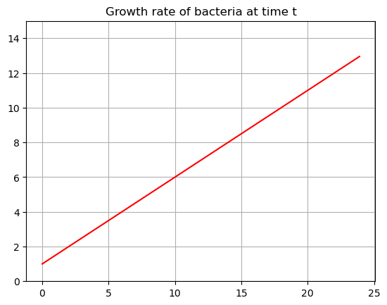
Now ask the same question
If I knew that at time \(t=0\) I had exactly \(5\) cells, how many cells would I have when \(t=10\)? How would I calculate this? Just using algebra and instincts:
- This one is a little harder because the function is changing.
- What rate should I pick?
- If I pick G(0) as the growth rate then it would say I have \(1\times10=10\) cells added or a total of \(15\) cells - underestimate
- If I pick G(10) it would say I have a growth of 6 cells per hour \(6\times 10 = 60\) cells added or a total of \(65\) cells- overestimate
Lets look at a graph
start=0
end=10
tfill = np.arange(start,end,0.1)
yfill1 = growth(0)*np.ones(len(tfill))
yfill2 = growth(10)*np.ones(len(tfill))


plt.plot(tdata,G,'-r')
plt.fill_between(tfill, yfill1, color='blue', alpha=0.7)
plt.fill_between(tfill, yfill2, color='lightgreen', alpha=0.7)
plt.title('Growth rate of bacteria at time t')
plt.ylim(0,15)
plt.grid()
plt.show()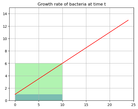
One of these is way under estimating and the other way over. The problem here is that the growth rate is changing continuously throughout the range. We can’t just easily pick a height. How could we do better?
- We could divide the range into two pieces and use two estimates for the rate of change. Lets use \(G(0)\) and \(G(5)\) as the estimates for the growth and then the base of our rectangle would be \(5\).
start=0
end=10
tfill1 = np.arange(start,end/2,0.1)
yfill1 = growth(0)*np.ones(len(tfill1))
tfill2 = np.arange(end/2,end,0.1)
yfill2 = growth(5)*np.ones(len(tfill2))


plt.plot(tdata,G,'-r')
plt.fill_between(tfill1, yfill1, color='lightblue', alpha=0.7)
plt.fill_between(tfill2, yfill2, color='lightgreen', alpha=0.7)
plt.title('Growth rate of bacteria at time t')
plt.ylim(0,15)
plt.grid()
plt.show()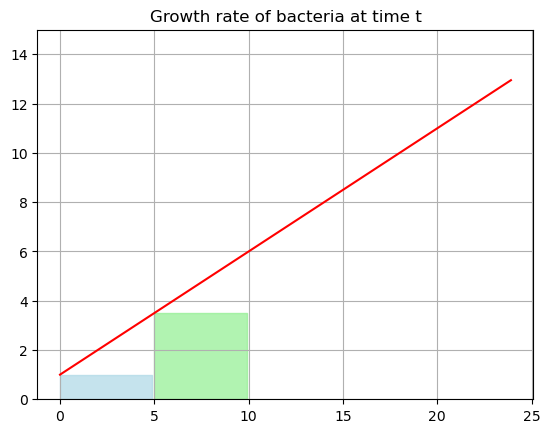
This is probably better, but still an underestimate.
\[B = G(0)(5)+G(5)(5)= 1(5)+3.5(5) = 22.5 \]
So we are estimating that we have \(5+22.5 = 27.5\) cells at time \(t=10\)
Well if we can divide twice we can divide 10 times, right?
start=0
end=10
N = 10

# Find the width of the base of the rectangles
# If we are dividing into ten sections then each rectangle has a base of (10-0)/10 =  1
delt = (end-start)/N
tvals = [start+i*delt for i in range(N)]

plt.plot(tdata,G,'-r')

bac = 5
# Loop through and add all those rectangles to the plot
for tval in tvals:
    tfill = np.arange(tval,tval+delt,0.01)
    yfill = growth(tval)*np.ones(len(tfill))
    plt.fill_between(tfill, yfill, color='gray', alpha=0.7)
    bac = bac + growth(tval)*delt

plt.title('Growth rate of bacteria at time t')
plt.ylim(0,15)
plt.grid()
plt.show()

print(f'Total bacterial at time 10 if we use {N} rectangles: {bac}')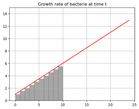
Total bacterial at time 10 if we use 10 rectangles: 37.5Wow, that got a lot better! What is our estimate now?
\[B = G(0)*\Delta t+G(1)*\Delta t+G(2)*\Delta t+\dots = 32.5 cells\]
where \(\Delta t\) is the width of the base of the rectangle, here \(\Delta t=1\). At \(t=10\) we would have \(32.5+5=37.5\) cells.
You Try - how can we get a better estimate?
- Rerun the code above to get a better estimate. You should only have to change the value of N!
Question
- As we increase N we are decreasing what?
- What is the general formula for adding up the rectangles (try to use summation notation it’s okay if it’s not perfect!)
- For a perfect answer we want the number of rectangles to go to what?
- What does this sound like we are doing?
.
.
.
.
.
.
Answers
- As we increase the number of rectangles we are decreasing the width of the rectangles - \(\Delta t\) is getting smaller. \[\Delta t = (tend-tstart)/N\]
- To add these things up we are doing a sum \[\sum_{i=0}^{N} G(t_i)\Delta t\] where we are taking the \(t\) value from the left hand side of the function. We could have just as easily taken this \(t\) value from the right side or even the middle somewhere.
- To get a perfect answer we would want an infinite number of rectangles with infinitesimal width!
- This is a LIMIT!!! \[\lim_{N\to\infty}\]
Integral Definition
We define the integral as the limit as \(N\) goes to infinity of this sum (Reimann Sum)
\[ \int G(t) \, dt = \lim_{N \to \infty} \sum_{i=1}^{N} G(t_i^*) \Delta t \]
Lets use the integral to answer our question exactly!
Given that the rate of change in the number of cells at time \(t\) is
\[G(t) = \frac{t}{2}+1\]
If I knew that at time \(t=0\) I had exactly \(5\) cells, how many cells would I have when \(t=10\)?
How would I calculate this?
- Find \(B(t)\) using the integral - remembering that it will give us a family of functions (we will need to add \(+c\))
- Plug in our numbers to find the answer
# Enter the growth function symbolically
t = sp.symbols('t')
G = t/2+1

# Let sympy find the integral
sp.integrate(G,t)
\(\displaystyle \frac{t^{2}}{4} + t\)
This means that the amount of bacteria is given by the family of functions
\[B(t) = \frac{t^2}{4}+{t}+c\]
we would need to know how much we started with to solve for \(c\). But we do know this! \(B(0)=5\) when \(t=0\) we have \(5\) cells. PLUG THIS IN
\[B(0)=c=5\]
so for our particular problem
\[B(t) = \frac{t^2}{4}+{t}+5 \]
# Enter the bacteria function symbolically
B = t**2/4 + t +5
B
\(\displaystyle \frac{t^{2}}{4} + t + 5\)
We can answer the question by subbing in \(t=10\).
B.subs(t,10)\(\displaystyle 40\)
When \(t=10\) I will have \(40\) cells.
Because I have a general function \(B(t)\) I can actually answer the question for any time! I could easily change the function if I had a different starting value. Calculus gives me a lot of power and flexibility.
Lets plot our function:
# Enter the function numerically
tdata = np.arange(0,24,0.01)
Bdata = tdata**2/4 + tdata +5

plt.plot(tdata,Bdata,'-g')
plt.plot(10,40,'or')
plt.title('Amount of bacteria at time t')
plt.grid()
plt.show()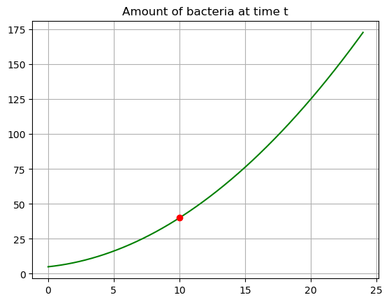
Integration - what do we know
- The integral of a function is related to the area under the curve.
- The solution to the integral is a family of functions where the \(+c\) represents the starting value, or the value at some point.
- The integral is the opposite of the derivative.
- It is a type of fancy addition - we are adding up the area under the curve of a changing function.
Example 3 - Non-Constant Rate of Change
Let’s take this a step further and use our original function
Let’s say I know the growth rate of some bacteria - maybe I got a bunch of data and modeled the growth rate over time.
\[ G(t) = 3(t-12)^2-10 \]
Now I want to use this information to predict the amount of bacteria in a sample at time \(t=10\) and I know that when \(t=0\) I had \(5\) cells. Here are my steps:
- Enter the growth function symbolically
- Use sympy to take the integral
- Find the constant of integration \(c\) using the information given.
- Construct the solution for your problem (particular soln)
- Answer the question.
we can do this all symbolically.
# 1. Enter the growth function
t = sp.symbols('t')
def growth(t):
    return 3*(t-12)**2-10

G = growth(t)
G
\(\displaystyle 3 \left(t - 12\right)^{2} - 10\)
# 2. Find the integral
B = sp.integrate(G,t)
print(B)
t**3 - 36*t**2 + 422*tTo find the constant:
\[B(t) = t^3 - 36t^2 + 422t + c\]
after I add my constant of integration. I plug in \(B(0)=5\)
\[B(0) = 0^3 - 36*0^2 + 422*0 + c\]
\[5 = (0)^3 - 36(0)^2 + 422(0) + c\]
so
\[ c = 5 - [(0)^3 - 36(0)^2 + 422(0)] \]
in sympy I could write this as
c = 5 - B.subs(t,0)# 3. Find the constant
tknown = 0
Bknown = 5
c = Bknown - B.subs(t,tknown)
c\(\displaystyle 5\)
# 4. Enter my B function with the added c
B = B + c
B
\(\displaystyle t^{3} - 36 t^{2} + 422 t + 5\)
# 5. Answer the question
B.subs(t,10)
\(\displaystyle 1625\)
Interpret Result
If my bacteria is growing at a rate given by \(G(t)\) and I start with \(5\) cells at time \(t=0\) then I will have \(1625\) cells ten hours later.
Visualization - extra
You don’t have to visualize the integral every time but it is important that you remember that it represents the area under the curve! We are adding up the growth function for every single teeny tiny narrow rectangle!
If you play with the code below you should see that as you increase \(N\) you get closer and closer to the real value of the integral!
start=0
end=10
N = 10

tdata=np.arange(0,24,0.01)
def growth(t):
    return 3*(t-12)**2-10
G = growth(tdata)

# Find the width of the base of the rectangles
# If we are dividing into ten sections then each rectangle has a base of (10-0)/10 =  1
delt = (end-start)/N
tvals = [start+i*delt for i in range(N)]

plt.plot(tdata,G,'-r')

# Starting bacteria amt
bac = 5

# Loop through and add all those rectangles to the plot
for tval in tvals:
    tfill = np.arange(tval,tval+delt,0.01)
    yfill = growth(tval)*np.ones(len(tfill))
    plt.fill_between(tfill, yfill, color='gray', alpha=0.7)
    bac = bac + growth(tval)*delt

plt.title('Growth rate of bacteria at time t')
plt.grid()
plt.show()

print(f'Total bacterial at time 10 if we use {N} rectangles: {bac}')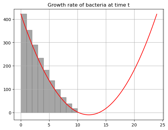
Total bacterial at time 10 if we use 10 rectangles: 1840.0You try
Solve the following problems using the integral. For each you should:
- Enter the growth function symbolically
- Use sympy to take the integral
- Find the constant of integration \(c\) using the information given.
- Construct the solution for your problem (particular soln)
- Answer the question.
Thanks to google gemini for the inspiration for these problems
A city’s water reservoir is experiencing varying inflow rates due to seasonal changes. The rate of water inflow, measured in cubic meters per day, is given by the function:
\[I(t)= 1500 + 300*sin(π*t/180)\]
where \(I\) is measured in cubic meters per day and \(t\) is measured in days.
- If the reservoir contained \(50,000\) cubic meters of water at \(t = 0\), determine the function representing the total volume of water in the reservoir at any time \(t\).
- Calculate the total volume of water that entered the reservoir between day 0 and day 90. Subtract the amount at \(t=0\) from the amount at \(t=90\).
- How much water should the city have on day 180?
A chemical reaction is producing heat at a rate that changes over time. The rate of temperature increase, measured in degrees Celsius per minute, is given by the function:
\[T(t) = = 0.8e^{-0.05t} + 0.1\]
- If the initial temperature at \(t = 0\) was \(25\) degrees Celsius, determine the function representing the temperature at any time \(t\).
- What is the temperature of the reaction after 30 minutes?
A factory’s production rate of a certain product is changing over time. The rate of production, measured in units per hour, is given by the function:
\[P(t) = 0.1t^2 - t + 10\]
where \(t\) is the time in hours between \(0\) and \(24\).
- If the factory had produced \(0\) units before time \(t=0\), determine the function representing the total number of units produced at any time \(t\).
- The cost of running the factory is given by the function \[C(t) = 0.5t^3\] and if we imagine that we can sell these products instantaneously for \(2\) dollars a piece then the profit is given by \[profit(t) = 2*units(t) - cost(t)\] based on your calculation above write down your profit function.
- At what time during the day is our profit maximized? Use what you know about derivatives to answer this question!
Integration and Data Science
In data science we don’t calculate integrals very often. What is far more important is the idea of what the integral stands for:
It finds the area under a curve
- probability - total area under curve is one
It is a way to do fancy addition of a continuously changing function
- signal processing
- probability
- certain cost functions rely on the idea of integration.
It is the opposite of the derivative
- If we know something about the rate of change in our data we can know about the original data.