# We will just go ahead and import all the useful packages first.
import numpy as np
import sympy as sp
import pandas as pd
import matplotlib.pyplot as plt
from mpl_toolkits.mplot3d import Axes3D

# Special Functions
from sklearn.metrics import r2_score, mean_squared_error

## NEW
from scipy.stats import binom, beta, norm

# Functions to deal with dates
import datetimeMath for Data Science
Hypothesis Testing
Important Information
- Email: joanna_bieri@redlands.edu
- Office Hours take place in Duke 209 unless otherwise noted – Office Hours Schedule
Today’s Goals:
- Normal Distribution
- Confidence Intervals
- Hypothesis Testing
(Review) Normal Distribution
- norm.pdf() - to see the normal curve - bell shaped, symmetrical
- np.mean() - to get the average of a set of numbers
- np.std() - to get the standard deviation of a set of numbers
- norm.cdf() - to get the cumulative distribution - integrate from 0 to xlim.
- norm.ppf() - to get the inverse cumulative distribution
- The probability density function for the normal distribution is given by
\[f(x) = \frac{1}{\sigma\sqrt{2\pi}}e^{-\frac{1}{2}\left(\frac{x-\mu}{\sigma}\right)^2}\]
Uniformly Distributed Variables - Normal Results
Last time we did an experiment where we were rolling dice. We know that each die has a uniform probability distribution. The chance of getting each number is \(1/6\). But when we added up more than one die being thrown, we saw something interesting happen. The sum of the numbers rolled seemed to follow the pattern of a normal distribution!
Below we sample uniformly distributed random numbers but in sets of 31 and then sum them (averaging would work too) - We see the result is a normal distribution!
num_rolls = 1000
num_dice = 31 # Number of dice rolled each time

# Set a random seed for reproducibility
np.random.seed(100)
sums = []
for _ in range(num_rolls):
    roll_results = np.random.randint(1, 8, num_dice) # Simulates dice rolls
    sums.append(np.sum(roll_results))

print(f'The mean is: {np.mean(sums)}')
print(f'The standard deviation is: {np.std(sums)}')

plt.hist(sums, bins=7, edgecolor='black')
plt.title("Simulated Sum of Dice Rolls")
plt.xlabel("Sum of Dice")
plt.ylabel("Frequency")
plt.show()
The mean is: 124.132
The standard deviation is: 10.99047660477015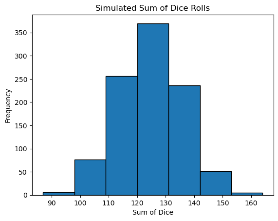
Keep this experiment in mind when we talk about the central limit theorem!
Inferential Statistics - Central Limit Theorem
Inferential statistics differs from descriptive statistics in that we hope to go beyond describing the data. In this case we use sample data to make inferences, predictions, and generalizations about a larger population. In data science we start with descriptive statistics as part of our exploratory data analysis (EDA), but in the longer term we hope to go beyond this and create predictions about whatever system we are considering.
BEWARE We are wired as humans to be biased and come quickly to conclusions, sometimes without considering all of the possible interactions, influences, or nuances in the data. Being a great data science professional means suppressing this desire to jump to conclusions and carefully consider what the data can actually tell you.
The Central Limit Theorem
Interesting things happen when we take large enough samples of a population, calculate the mean of each, and then plot the distribution.
- The mean of the sample means is equal to the population mean.
- If the population is normal, then the sample means will be normal.
- If the population is not normal, but the sample size is greater than 30, the sample means will still roughly form a normal distribution.
- The standard deviation of the sample means equals the population standard deviation divided by the square root of the sample size.
\[ sample\:standard\:deviation = \frac{population\:standard\:deviation}{\sqrt{sample\:size}}\]
What does this do for us? We can now infer things about populations based on samples - even if the underlying distribution is not normal!!!
31 is a textbook number for when our sample distribution often converges onto the population distribution. If you have fewer than 31 samples then you need to rely on a different distribution (the T-distribution).
Here is an article where you can learn more about how much of a sample really is enough:
https://www.dummies.com/article/academics-the-arts/math/statistics/the-central-limit-theorem-whats-large-enough-142651/
Confidence Intervals
Confidence intervals allow us to say how confidently we believe a sample mean (or another parameter) falls in a range for a population mean. How much do we believe the data for the sample is predictive of the population. Remember:
- Sample - The data I collected. I try to get a good representative sample, but usually I cannot get data for the WHOLE population.
- Population - The real world system. This is what I want to know about based on the sample data I collected.
Example: Golden Retrievers We looked at data about golden retriever weights last class. Here is something we can say:
*Based on a sample of 31 golden retrievers with a sample mean of 65.405 and a standard deviation of 5.36, I am 95% confident that the population mean lies between 63.92 and 66.89.
We will build up this argument/calculation in steps.
# Here is some code that will load the data for us
data = pd.read_csv('https://joannabieri.com/mathdatascience/data/goldenweights.csv')
golden_retriever_weights = list(data['weight'])

# Make a line plot
y = np.zeros(len(golden_retriever_weights))
plt.figure(figsize=(10, 2))  # Adjust figure size as needed
plt.scatter(golden_retriever_weights, y, s=100, marker='o', color='black',alpha=.5) #plot points
plt.yticks([])  # Hide y-axis ticks
plt.xlabel("Golden Retriever Weights")
plt.axhline(0, color='black', linewidth=0.8) #draw the numberline
plt.grid(True, axis='x', linestyle='--', alpha=0.6) #add grid for x-axis
plt.show()

mu = np.mean(golden_retriever_weights)
sigma = np.std(golden_retriever_weights)
print(f'The average is: {mu}')
print(f'The standard deviation is: {sigma}')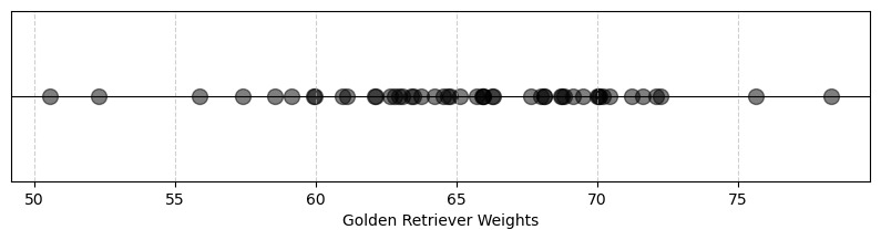
The average is: 65.405043722571
The standard deviation is: 5.3610122946938406
Level of Confidence (LOC)
We start by choosing how confident we need to be in our answer. This level of confidence can depend on how much error tolerance you have in real world system. 95% confidence is a good baseline - but this can depend on your application.
Z-scores
The Z-score has the following formula
\[z=\frac{x-\mu}{\sigma}\]
where \(\mu\) is the sample mean and \(\sigma\) is the standard deviation. This variable can be used to rescale a given distribution into the standard normal distribution (centered at 0 with a std of 1). This can help us compare data from two different distributions.
Here we will use it to find boundaries!
Critical Z-value - Symmetrical Probability in the Center
It this case we are seeking a Critical Z-value - this gives us a symmetrical range around the mean of our standard normal distribution that matches the cutoff for 95% confidence. Lets look at a picture of this!
confidence = .95
lower = (1-confidence)/2
upper = 1-lower
a = norm.ppf(lower,0,1)
b = norm.ppf(upper,0,1)


# Generate x values (range from 0 to 1)
x = np.linspace(-4, 4, 100)
# Calculate the probability density function (PDF)
pdf = norm.pdf(x, 0, 1)

plt.plot(x,pdf,'-k')

# Color in the area under the curve from 0 to 0.9
x_fill = np.linspace(a, b, 100)
pdf_fill = norm.pdf(x_fill, 0, 1)
plt.fill_between(x_fill, pdf_fill, color='lightblue', alpha=0.7, label='Area up to 0.9')

plt.title(f'Standard Normal Distribution with {confidence} percent confidence colored in.')
plt.xlabel('x')
plt.ylabel(f'Probability')
plt.grid()
plt.show()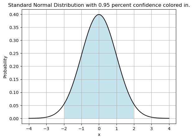
a-1.959963984540054b1.959963984540054This tells me that 95% of my probability is between -1.959963984540054 and 1.959963984540054 for the standard normal distribution. So our critical z-value is
\[z_c = 1.959963984540054\]
Notice in the code, the edges of my confidence interval are the x-locations given by the inverse cumulative distribution function at locations \(p=.025\) and \(p=.975\) so that only 5% of the data is outside this range - chopping off 2.5$ on each tail.
Margin of Error
So what we have so far is the cutoffs on the edge of the normal distribution that serves as a boundary for 95% of our probability. The margin of error formula is given by
\[ E = \pm z_c \frac{\sigma}{\sqrt{n}}\]
here \(z_c\) are the critical z-values found above, \(\sigma\) is the standard deviation, and \(n\) is the sample size.
z_c = 1.959963984540054
sigma = np.std(golden_retriever_weights)
n = 50

E = z_c*sigma/np.sqrt(n)
E1.4859694883203671Then we can apply this margin of error to the sample mean.
\[ 65.405043722571 \pm 1.4859694883203671 \]
Or say that we are 95% certain that the average weight in our population is between 63.92 and 66.89.
Here is some code that will do the full calculation for you.
confidence = .95

# Get the mean and standard deviation of the sample
mu = np.mean(golden_retriever_weights)
sigma = np.std(golden_retriever_weights)

# Get the sample size
n = len(golden_retriever_weights)

# Get the critical z_c = [a,b] for your confidence LOC
# from the standard normal distribution
lower = (1-confidence)/2
upper = 1-lower
# These will match a=-b
a = norm.ppf(lower,0,1)
b = norm.ppf(upper,0,1)

# Calcuate the margin of error
z_c = b # Use the positive one
E = z_c*sigma/np.sqrt(n)

# Apply this to the mean
UPPER = mu+E
LOWER = mu-E

print(f'I am {confidence*100}% certain that the population mean is between {LOWER} and {UPPER}.')
I am 95.0% certain that the population mean is between 63.91907423425063 and 66.89101321089136.You Try
Redo the example above except this time try a different LOC or confidence interval. Try 99% and 75% confidence. Then interpret your results. Do the ranges for the mean weight make sense?
P-values and Hypothesis Testing
When we say something is statistically significant, what the heck does that even mean? The idea behind statistical significance is that we want to know what is the probability that our results were random chance vs what is the probability that there is some pattern or evidence in our data. Here is the historical story:
In 1920s Cambridge, Muriel Bristol was a Botanist who claimed she could discern whether milk or tea was poured first into a cup. Statistician Ronald Fisher designed an experiment with eight randomized cups, four of each type, to test her claim. Dr. Bristol was able to identify all of them correctly. So Dr. Fisher asked “what is the chance of this happening randomly”? It turns out it is a 1 in 70 chance, or 1.4% probability that this result happened randomly rather than by the hypothesized explanation (Hypothesis - Dr. Bristol really could tell the difference). This is what we call the p-value.
Traditionally the threshold for statistical significance is a p-value of 5%. How does this work: 1. Make your hypothesis (alternative hypothesis) (Dr. Bristol can tell the difference - random luck did not play a significant role - the variable in question is causing a positive result.) 2. Make your null-hypothesis (The results were random chance - random luck played a role - something else is happening here - the variable in question is not causing the positive result) 3. Find your p-value - if it is less then .05 we can reject the null hypothesis.
Example
The population of people with a cold has a mean recovery time of 18 days, with a standard deviation of 1.5 days, and follows a normal distribution. This means that there is a 95% chance that recovery will take between 15-21 days.
How was this calculated
mean = 18
stdev = 1.5

upper = 21
lower = 15

x = norm.cdf(upper,mean,stdev) - norm.cdf(lower,mean,stdev)

print(f'Percent of the data between {upper} and {lower} is {x*100}%')
Percent of the data between 21 and 15 is 95.44997361036415%This also means there is less than a 2.5% chance of our recovery time being outside this range.
Let’s say that you are experimenting on a new drug that was given to a group of 32 people, and it took an average of 16 days for them to recover from the cold. You want to know if the drug had an impact or if you could have just randomly chosen really quick healing people. Other ways to frame this question:
- Does the drug show a statistically significant results?
- Was the 16 day average recovery just a coincidence?
Null Hypothesis (Nothing is happening here) The 16 day average was just a coincidence.
Alternative Hypothesis (Something is happening here) The drug did have an effect.
One tailed test
Here we will frame our null and alternative hypothesis using inequalities.
- The null hypothesis would say that the population mean is greater than or equal to 18 (the number given in past studies).
- The alternative hypothesis would say the population mean is less than 18.
To reject the null hypothesis we would need to show that the sample mean of the test subjects was likely to have been random chance. We will use the traditional p-value of \(0.05\) for our test. Here is how we will do the test:
- Ask what the cutoff is for statistical significance being careful to take into account the sample size.
- We will compare this to the mean that we found in our study and evaluate the inequalities or check to see if our p-value is below 0.05
# Data from past studies
population_mean = 18
population_stdev = 1.5

# Data for our hypothesis test
p = 0.05
sample_mean = 16
sample_size = 32
SEM = population_stdev/np.sqrt(sample_size) # This is the Standard Error of the Mean SEM

# Get the z-value
z = (sample_mean-population_mean)/SEM
print(f'Our z-value is {z}')

# Use the use the cumulative distribution function for the standard normal to see
# The probability of getting a z-score less than the one you got.
p_value = norm.cdf(z,0,1)

# Compare the results
print(f'For our results to be statistically significant our p-value: {p_value} to be less than the cutoff p: {p}.')
Our z-value is -7.542472332656508
For our results to be statistically significant our p-value: 2.3057198811629587e-14 to be less than the cutoff p: 0.05.What is the critical recovery time cutoff under which we would say that the results are significant?
# This is the same as what we found above for the Error
# This is the negative side since p=0.05
z_c = norm.ppf(p,0,1)

# Find what recovery time matches this
x_c = population_mean + z_c*SEM
print(f'In this study with {sample_size} samples we would need to see a mean recovery time of {x_c} or below to have statistically significant results.')
In this study with 32 samples we would need to see a mean recovery time of 17.563842317371247 or below to have statistically significant results.Our study mean was 16 which was smaller than 17.5638 so we reject the null hypothesis.
Our p-value was nearly zero which is less than 0.05 so we reject the null hypothesis.
The results of the p-test indicate that the new drug significantly reduces the recovery time for people with a cold.
BEWARE The one tailed test only checks if our mean is below some cutoff… so if our drug actually made things WORSE, our results would be that the drug had no impact! This is why we almost always use the two tailed test.
Two Tailed Test
In the above experiment we looked for significance in only one tail of the distribution. It is usually better practice to look at a two-tailed test, considering both tails of the distribution. Using the same data, we can reframe our hypothesis in terms of equalities.
- The null hypothesis would say that the population mean is equal to 18.
- The alternative hypothesis would say the population mean not equal to 18.
Here notice that instead of saying our drug has an impact in one direction (it improves our mean recovery time) we are looking at whether our drug had any effect at all (positive or negative). In this case we are spreading our p-value into both tails of the distribution and considering the area outside the central 95% of the normal distribution.
- Ask what the cutoff is for statistical significance being careful to take into account the sample size - on the left tail (2.5%)
- Ask what the cutoff is for statistical significance being careful to take into account the sample size - on the right tail (97.5%)
- Consider whether our results are outside of these ranges or whether our p value is below 0.05.
# Data from past studies
population_mean = 18
population_stdev = 1.5

# Data for our hypothesis test
p = 0.05
sample_mean = 16
sample_size = 32
SEM = population_stdev/np.sqrt(sample_size) # This is the Standard Error of the Mean SEM

# Get the z-value
z = (sample_mean-population_mean)/SEM
print(f'Our z-value is {z}')

# THIS IS SLIGHTLY DIFFERENT!
# Use the use the cumulative distribution function for the standard normal to see
# The probability of getting a z-score less than the one you got on one side
p_left = norm.cdf(z,0,1)
# The probability of getting a z-score greater than the one you got on the other side
p_right = 1-norm.cdf(-z,0,1)
p_value = p_right+p_left


# Compare the results
print(f'For our results to be statistically significant our p-value: {p_value} to be less than the cutoff p: {p}.')
Our z-value is -7.542472332656508
For our results to be statistically significant our p-value: 4.6149837723832843e-14 to be less than the cutoff p: 0.05.Again we see that our result is statistically significant, but our p value is larger. This is because this test split the probability that we are outside the 95% to both tails.
What are the critical x-values that we would need to be between to get statistically significant results?
# This is the same as what we found above for the Error
# This is the negative side since p=0.05
# We do p/2 because we are splitting the tails on either side
z_c = norm.ppf(p/2,0,1)

# Find what recovery time matches this
x_c_right = population_mean - z_c*SEM
x_c_left = population_mean + z_c*SEM
print(f'In this study with {sample_size} samples we would need to see a mean recovery time outside {x_c_left} and {x_c_right} to have statistically significant results.')
In this study with 32 samples we would need to see a mean recovery time outside 17.48028606586887 and 18.51971393413113 to have statistically significant results.We see that our study mean was outside the cutoffs, so so our results are statistically significant. This test would also tell us if the drug had a negative effect!
Notice The two tailed test sets a higher standard for statistical significance. It makes it harder to reject the null. We also often care about whether or not our mean was shifted in either direction. Two tailed tests tend to be more reliable and are preferable in most cases.
Beware of p-Hacking! P-hacking, or data dredging, is when researchers manipulate their data or analysis to find a statistically significant result (a low p-value) even if one doesn’t truly exist. This can involve things like stopping data collection early, removing outliers, or trying many different analyses until a “significant” result appears. While tempting, p-hacking leads to unreliable and often false conclusions, undermining the integrity of scientific research.
You Try
How would the results change if you had more or fewer samples?
You Try
Harvest Table claims their chocolate chip cookies have an average of 12 chocolate chips per cookie. You, being a dedicated cookie connoisseur, suspect they’re exaggerating! You decide to investigate.
Part 1: Sampling and the Normal Distribution
Sample Collection: You secretly purchase 50 cookies over a week and count the number of chocolate chips in each. Here are your results:
cookie_counts = [10, 12, 11, 12, 10, 11, 17, 15, 14, 13,  9, 10, 14, 14,  9,  9, 16,
       11, 11, 13, 12, 13, 14,  8, 16, 13, 11, 10, 11, 13, 10,  9, 12, 11,
       13, 11, 14, 11, 14, 10, 11,  9, 14, 12,  8, 16, 14,  9, 11, 10]
print(cookie_counts)
[10, 12, 11, 12, 10, 11, 17, 15, 14, 13, 9, 10, 14, 14, 9, 9, 16, 11, 11, 13, 12, 13, 14, 8, 16, 13, 11, 10, 11, 13, 10, 9, 12, 11, 13, 11, 14, 11, 14, 10, 11, 9, 14, 12, 8, 16, 14, 9, 11, 10]- Calculate:
- Find the sample mean and sample standard deviation of your data.
- Assuming the population of chocolate chips per cookie is normally distributed, plot a graph of the normal distribution using your sample mean and standard deviation.
Part 2: Confidence Intervals
Calculate: Construct a 95% confidence interval for the sampled average number of chocolate chips per cookie. You will need to calculate the margin of error here.
Interpret: What does this confidence interval tell you?
Part 3: Hypothesis Testing and P-Values
- Formulate:
- State the null hypothesis and alternative hypothesis.
- Calculate:
- Find the p-value associated with your data. Do the two tailed test. Here the SEM will use the sample standard deviation since we don’t have the population standard deviation.
- Interpret:
- If you’re using a significance level of 0.05, do you reject or fail to reject the null hypothesis?
- What does the p-value tell you about the strength of evidence against the Harvest Table’s claim?
- Write a short conclusion in the context of the cookie caper. Did the Harvest Table exaggerate?
Bonus:
- Discuss potential sources of error in your sampling or analysis.
- What would you do differently if you were to conduct this experiment again?
Code
num_samples = len(cookie_counts)

# Normal Distribution
sample_mean = np.mean(cookie_counts)
sample_std = np.std(cookie_counts)

print(f"Sample Mean: {sample_mean}")
print(f"Sample Standard Deviation: {sample_std}")

# Plot the Normal Distribution for our Data
x_vals = np.linspace(0,24,1000)
pdf = norm.pdf(x_vals,sample_mean,sample_std)

plt.plot(x_vals,pdf,'-k')
plt.grid()
plt.show()

# Part 2: Confidence Intervals and Margin of Error
confidence = 0.95
# Get the critical z_c = [a,b] for your confidence LOC
# from the standard normal distribution
lower = (1-confidence)/2
upper = 1-lower
# These will match a=-b
a = norm.ppf(lower,0,1)
b = norm.ppf(upper,0,1)

# Calcuate the margin of error
z_c = b # Use the positive one
E = z_c*sample_std/np.sqrt(num_samples)
# Apply this to the mean
UPPER = sample_mean+E
LOWER = sample_mean-E

print(f'I am {confidence*100}% certain that the sample mean is between {LOWER} and {UPPER}. This does not tell me how I directly compare with the assumed population mean.')

print(f'My null hypothesis is that the mean is equal to 12.')
print(f'My alternative hypothesis is that the mean is not equal to 12.')
Sample Mean: 11.82
Sample Standard Deviation: 2.2062638101550776
I am 95.0% certain that the sample mean is between 11.208466109596358 and 12.431533890403642. This does not tell me how I directly compare with the assumed population mean.
My null hypothesis is that the mean is equal to 12.
My alternative hypothesis is that the mean is not equal to 12.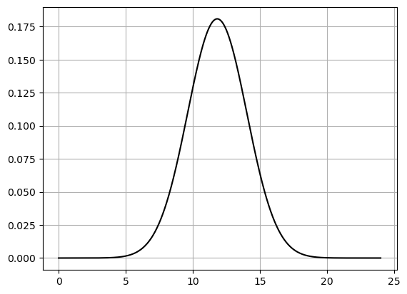
Code
# Data from past studies
population_mean = 12

# Data for our hypothesis test
p = 0.05
sample_size = 50
SEM = sample_stdev/np.sqrt(sample_size) # This is the Standard Error of the Mean SEM

# Get the z-value
z = (sample_mean-population_mean)/SEM
print(f'Our z-value is {z}')

# TWO SIDED TEST
p_left = norm.cdf(z,0,1)
p_right = 1-norm.cdf(-z,0,1)
p_value = p_right+p_left
# NOTE WE CAN ALSO JUST DO 2*p_right... since this is symmetric

# Compare the results
print(f'For our results to be statistically significant our p-value: {p_value} to be less than the cutoff p: {p}.')


# This is the same as what we found above for the Error
# This is the negative side since p=0.05
# We do p/2 because we are splitting the tails on either side
z_c = norm.ppf(p/2,0,1)

# Find what recovery time matches this
x_c_right = population_mean - z_c*SEM
x_c_left = population_mean + z_c*SEM
print(f'In this study with {sample_size} samples we would need to see a mean number of chips outside {x_c_left} and {x_c_right} to have statistically significant results.')
Our z-value is -0.6151985873962956
For our results to be statistically significant our p-value: 0.5384235805689417 to be less than the cutoff p: 0.05.
In this study with 50 samples we would need to see a mean number of chips outside 11.426537179302805 and 12.573462820697195 to have statistically significant results.