# We will just go ahead and import all the useful packages first.
import numpy as np
import sympy as sp
import pandas as pd
import matplotlib.pyplot as plt
from mpl_toolkits.mplot3d import Axes3D

# Special Functions
from sklearn.metrics import r2_score, mean_squared_error

## NEW
from scipy.stats import binom, beta, norm

# Functions to deal with dates
import datetimeMath for Data Science
Exam Review - Probability
Important Information
- Email: joanna_bieri@redlands.edu
- Office Hours take place in Duke 209 unless otherwise noted – Office Hours Schedule
Today’s Goals:
- Review topics from Probability for our Exam
This lab is inspired by a chat with Google Gemini. My Prompt: Can you help me come up with a python lab that will help my students study for a data science exam in probability. I would like to start with a data set and have them answer questions about joint, union, and conditional probabilities, the binomial distribution, the beta distribution, and the normal distribution.
I then updated the data and questions to better suit our class and be more interesting, in my opinion!
## Get the data
file = 'data/student_stress.csv'
data = pd.read_csv(file)data| Stress_Level | Art_Club | Sports_Club | Both_Clubs | |
|---|---|---|---|---|
| 0 | 5.993428 | True | True | True |
| 1 | 4.723471 | True | True | True |
| 2 | 6.295377 | False | True | False |
| 3 | 8.046060 | False | False | False |
| 4 | 4.531693 | True | False | False |
| ... | ... | ... | ... | ... |
| 995 | 4.437799 | True | False | False |
| 996 | 8.595373 | True | False | False |
| 997 | 6.281686 | False | False | False |
| 998 | 3.857642 | True | False | False |
| 999 | 6.145166 | True | True | True |
1000 rows × 4 columns
# To just get the art club I type
data['Art_Club']
0 True
1 True
2 False
3 False
4 True
...
995 True
996 True
997 False
998 True
999 True
Name: Art_Club, Length: 1000, dtype: bool# To count the number of true
sum(data['Art_Club'])383# To count the total number
len(data['Art_Club'])1000Part 1 - Probabilities from Data
Marginal Probabilities Calculate these directly from the data.
- What is the probability that a student participates in Art?
- What is the probability that a student participates in Sports?
- What is the probability that a student participates in Both?
Joint, Union, and Conditional Probabilities
- Write down the general formula for Joint Probabilities and notice that above you have found P(A), P(S), and P(A and S) from the data. Use this information to find the conditional probability P(A|S).
- Write down Bayes’ Theorem and use it to calculate P(S|A).
- Interpret these results. Eg. is it more likely for a Sports student to do art or an art student to do sports?
- Write down the general formula for Union Probabilities. What is the probability that is student is in either Art or Sports?
#1
P_A = sum(data['Art_Club'])/len(data)
#2
P_S = sum(data['Sports_Club'])/len(data)
#3
P_B = sum(data['Both_Clubs'])/len(data)

print(f'P(A) = {P_A},   P(S) = {P_S},   P(B) = {P_B}')
P(A) = 0.383, P(S) = 0.306, P(B) = 0.11Joint Probability
\[P(A\; and\; B) = P(B)\times P(A|B)\]
we cal solve this for \(P(A|B)\) in my case A=Art and B=Sports
#4
P_A_given_S = P_B/P_S
print(f'P(A|S) = {P_A_given_S}')
P(A|S) = 0.35947712418300654Bayes Theorem
\[ P(A|B) = \frac{P(B|A)P(A)}{P(B)}\]
I have \(P(A|S)\) and I want to solve for \(P(S|A)\)
#5
P_S_given_A = P_A_given_S*P_S/P_A
print(f'P(S|A) = {P_S_given_A}')
P(S|A) = 0.28720626631853785#6
From this I see that it there is a 35.9% probability that a student in sports also participates in art and a 28.7% probability that a student in art also participates in sports. So it is more likely that a student in sports participates in art.
Union Probability
\[P(A\; or\; B) = P(A)+P(B) - P(B)\times P(A|B)\]
#7
P_A_or_B = P_A+P_S-(P_S*P_A_given_S)
print(f'P(A or B) = {P_A_or_B}')
P(A or B) = 0.5790000000000001Part 2
Binomial Distribution
- Assume the probability of a student participating in Art Club is a fixed value (e.g., the observed probability from the dataset that you found above). If we randomly select 15 students, what is the probability that exactly 6 of them participate in Art Club?
- Plot the probability distribution (binomial) for the number of students participating in art (from 0 to 15)
Beta Distribution
- Suppose we want to model our belief about the probability of a student participating in Sports Club. We observe the number of students who participate and do not participate. Using the data for number of students in sports, how many successes (participate in sports) vs failures (do not participate in sports) do we see in the data?
- Use the successes and failures you found above to plot the beta distribution.
- Find the probability that the underlying probability of students being in the sports club is what we found above. Interpret your result.
Normal Distribution
- Find the mean and standard deviation of student stress levels.
- Plot a histogram of student stress levels. Is it plausible that this follows a normal distribution? Explain why you think this.
- Find the error for 95% confidence in the mean stress levels.
Hypothesis Testing
Assume that the population of students from our school has a mean stress level of 5 with a standard deviation of 0.2, and follows a normal distribution.
Based on the data sample above, does participating in both clubs reduce a students stress level? In other words is the sample mean significantly different from the population mean? First get the data for only the students who participate in both clubs and find their mean and standard deviation of stress levels.
art_stress = data[data['Both_Clubs']==True]['Stress_Level']Create the alternative and null hypothesis.
Do a two tailed test to see if the change in the mean is statistically significant. Talk about both the p-values and the x cutoffs.
Interpret/Explain your results
#1
n = 15
p = P_A
k = 6

six_of_fifteen = binom.pmf(k,n,p)
print(f'The probability that exactly 6 of 15 randomly chosen students participate in Art = {six_of_fifteen}')
The probability that exactly 6 of 15 randomly chosen students participate in Art = 0.20472138071417764n = 15 # Number of Trials
p = P_A # Probability of Success
flip_binom = []
k_vals = []
for k in range(n+1):
k_vals.append(k)
P = binom.pmf(k,n,p)
flip_binom.append(P)
print(f'k={k}: P(X={k})={P}')
plt.bar(k_vals,flip_binom)
plt.title('Probability Mass - Participation in Art')
plt.xlabel(f'k outcomes in n={n} trials')
plt.ylabel('Probability')
plt.show()k=0: P(X=0)=0.0007149529467684289
k=1: P(X=1)=0.0066570578268794495
k=2: P(X=2)=0.028926372826359525
k=3: P(X=3)=0.07780897369121785
k=4: P(X=4)=0.1448987208609549
k=5: P(X=5)=0.1978795173378293
k=6: P(X=6)=0.20472138071417764
k=7: P(X=7)=0.16338842308908796
k=8: P(X=8)=0.1014226354021405
k=9: P(X=9)=0.04896706024007539
k=10: P(X=10)=0.01823765063722746
k=11: P(X=11)=0.005145881975878967
k=12: P(X=12)=0.0010647611003574522
k=13: P(X=13)=0.00015252593246611548
k=14: P(X=14)=1.3525684680370985e-05
k=15: P(X=15)=5.597338987122726e-07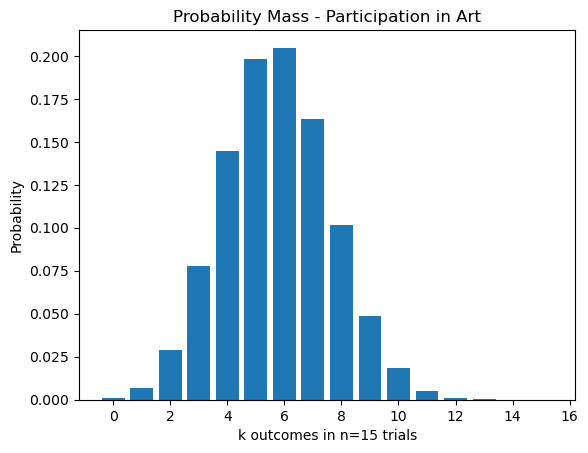
#3

successes = sum(data['Sports_Club'])
failures = len(data)-successes

print(f'We have {successes} successes and {failures} failures')
We have 306 successes and 694 failures#4
alpha_val = 306
beta_val = 694
# Generate x values (range from 0 to 1)
x = np.linspace(0, 1, 100)
# Calculate the probability density function (PDF)
pdf = beta.pdf(x, alpha_val, beta_val)
plt.plot(x,pdf,'-k')
plt.title(f'beta Distribution with alpha={alpha_val} and beta={beta_val}')
plt.xlabel('Underlying Rate of Success')
plt.ylabel(f'Likelihiid of {alpha_val}/{alpha_val+beta_val} successes')
plt.grid()
plt.show()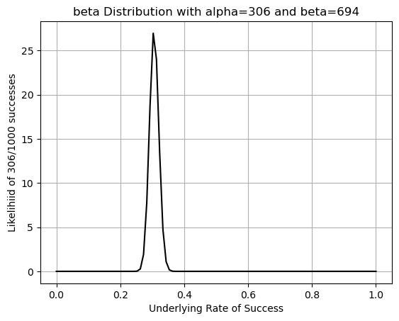
#5
beta.cdf(P_S,alpha_val,beta_val)
print(f'There is a 50.3% probability that the percent of students who will join the Sports Club reall is {P_S}.')
There is a 50.3% probability that the percent of students who will join the Sports Club reall is 0.306.#6
stress_level = data['Stress_Level']
mu = np.mean(stress_level)
sigma = np.std(stress_level)
print(f'The average stress level is {mu}')
print(f'The standard deviation of the stress levels is {sigma}')The average stress level is 5.0386641116446516
The standard deviation of the stress levels is 1.9574524154947084#7
plt.hist(stress_level, bins=10, edgecolor='black')
plt.title("Distribution of Student Stress Levels")
plt.xlabel("Stress Level")
plt.ylabel("Frequency")
plt.grid(True)
plt.show()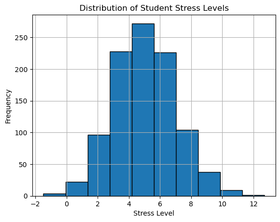
#7 Continued
print('First - this totally looks like a normal distribution')
print('But we could also do the test')

      # Check if our data is normally distributed
num_std = [1,2,3]

for n in num_std:
    # Get the range +- n standard deviations
    upper = mu+n*sigma
    lower = mu-n*sigma
    # Count up the data
    count = 0
    for d in stress_level:
        if d < upper and d>lower:
            count+=1
    print(f'Within {n} standard deviations we have {count/len(stress_level)*100} percent of the data')
First - this totally looks like a normal distribution
But we could also do the test
Within 1 standard deviations we have 68.60000000000001 percent of the data
Within 2 standard deviations we have 95.6 percent of the data
Within 3 standard deviations we have 99.7 percent of the data#8
confidence = .95
# Get the mean and standard deviation of the sample
mu = np.mean(stress_level)
sigma = np.std(stress_level)
# Get the sample size
n = len(stress_level)
# Get the critical z_c = [a,b] for your confidence LOC
# from the standard normal distribution
lower = (1-confidence)/2
upper = 1-lower
# These will match a=-b
a = norm.ppf(lower,0,1)
b = norm.ppf(upper,0,1)
# Calcuate the margin of error
z_c = b # Use the positive one
E = z_c*sigma/np.sqrt(n)
# Apply this to the mean
UPPER = mu+E
LOWER = mu-E
print(f'I am {confidence*100}% certain that the population mean is between {LOWER} and {UPPER}.')I am 95.0% certain that the population mean is between 4.917342183335033 and 5.15998603995427.#9
both_stress = data[data['Both_Clubs']==True]['Stress_Level']
mu_new = np.mean(both_stress)
sigma_new = np.std(both_stress)
print(f'The average stress level for students in Both Clubs is {mu_new}')
print(f'The standard deviation of the stress levels for students in Both Clubs is {sigma_new}')The average stress level for students in Both Clubs is 4.755903332990052
The standard deviation of the stress levels for students in Both Clubs is 2.0791692491190856#10
alternative hypothesis - participating in both clubs changes the stress level so the mean will not be equal to 5
null hypothesis - participating in both clubs does not change the stress level so the mean will be equal to 5
#11
# Data from past studies
population_mean = 5
population_stdev = 0.2

# Data for our hypothesis test
p = 0.05
sample_mean = mu_new
sample_size = len(both_stress)
SEM = population_stdev/np.sqrt(sample_size) # This is the Standard Error of the Mean SEM

# Get the z-value
z = (sample_mean-population_mean)/SEM
print(f'Our z-value is {z}')

# THIS IS SLIGHTLY DIFFERENT!
# Use the use the cumulative distribution function for the standard normal to see
# The probability of getting a z-score less than the one you got on one side
p_left = norm.cdf(z,0,1)
# The probability of getting a z-score greater than the one you got on the other side
p_right = 1-norm.cdf(-z,0,1)
p_value = p_right+p_left


# Compare the results
print(f'For our results to be statistically significant our p-value: {p_value} to be less than the cutoff p: {p}.')
Our z-value is -12.800537208443808
For our results to be statistically significant our p-value: 8.141047639847396e-38 to be less than the cutoff p: 0.05.# This is the same as what we found above for the Error
# This is the negative side since p=0.05
# We do p/2 because we are splitting the tails on either side
z_c = norm.ppf(p/2,0,1)
# Find what recovery time matches this
x_c_right = population_mean - z_c*SEM
x_c_left = population_mean + z_c*SEM
print(f'In this study with {sample_size} samples we would need to see a mean recovery time outside {x_c_left} and {x_c_right} to have statistically significant results.')In this study with 110 samples we would need to see a mean recovery time outside 4.962624953289446 and 5.037375046710554 to have statistically significant results.#12
Our results are statistically significant! There is enough evidence with a sample of 110 students that participation in both clubs changes the stress from the mean of 5. Since the stress levels are less for the students in both clubs. There is evidence that participation in both clubs reduces stress.