Math for Data Science

Linear Algebra and Matrices

Important Information

• Email: joanna_bieri@redlands.edu
• Office Hours take place in Duke 209 unless otherwise noted – Office Hours Schedule

Today’s Goals:

• Vectors continued
• Introducing Matrices
• Multiplication and Determinants
• Linear Programming

# We will just go ahead and import all the useful packages first.
import numpy as np
import sympy as sp
import pandas as pd
import matplotlib.pyplot as plt
from mpl_toolkits.mplot3d import Axes3D

# Special Functions 
from sklearn.metrics import r2_score, mean_squared_error
from sklearn.neighbors import KNeighborsClassifier
from scipy.stats import binom, beta, norm

# Functions to deal with dates
import datetime

# Some helpful functions for visualizations today
def plot_vector(vector,origin=(0, 0), color='b', label=None):
    """Plots a vector from the origin."""
    plt.quiver(origin[0], origin[1], vector[0], vector[1], 
               angles='xy', 
               scale_units='xy', 
               scale=1, 
               color=color, 
               label=label, 
               headwidth=3, 
               headlength=4)
    # Autoscale the axes based on the vectors
    all_x = [0, vector[0]]
    all_y = [0, vector[1]]
    min_x = min(all_x) - 1 
    max_x = max(all_x) + 1
    min_y = min(all_y) - 1
    max_y = max(all_y) + 1
    plt.xlim(min_x, max_x)
    plt.ylim(min_y, max_y)
    plt.xlabel('x')
    plt.ylabel('y')
    plt.title('Vector Plot')
    plt.grid(True)

def vector_addition(v1, v2):
    """Adds two vectors and plots the result."""
    result = v1 + v2
    plot_vector(v1, color='b', label='v1')
    plot_vector(v2,origin=(v1[0],v1[1]), color='g', label='v2')
    plot_vector(result, color='r', label='v1 + v2')
    plt.legend(loc='upper left', bbox_to_anchor=(1, 1))
    # Autoscale the axes based on the vectors
    all_x = [0, v1[0], v2[0], v1[0] + v2[0]]
    all_y = [0, v1[1], v2[1], v1[1] + v2[1]]
    min_x = min(all_x) - 1 
    max_x = max(all_x) + 1
    min_y = min(all_y) - 1
    max_y = max(all_y) + 1
    plt.xlim(min_x, max_x)
    plt.ylim(min_y, max_y)
    plt.title('Vector Addition')
    plt.grid(True)
    plt.show()
    return result

def vector_subtraction(v1, v2):
    """Subtracts v2 from v1 and plots the result."""
    result = v1 - v2
    plot_vector(v1, color='b', label='v1')
    plot_vector(v2, color='g', label='v2')
    plot_vector(result,origin=(v2[0],v2[1]), color='m', label='v1 - v2')
    plt.legend(loc='upper left', bbox_to_anchor=(1, 1))
    plt.title('Vector Subtraction')
    plt.grid(True)
    # Autoscale the axes based on the vectors
    all_x = [0, v1[0], v2[0], v1[0] - v2[0]]
    all_y = [0, v1[1], v2[1], v1[1] - v2[1]]
    min_x = min(all_x) - 1 
    max_x = max(all_x) + 1
    min_y = min(all_y) - 1
    max_y = max(all_y) + 1
    plt.xlim(min_x, max_x)
    plt.ylim(min_y, max_y)
    plt.axhline(0, color='black', linewidth=0.5)
    plt.axvline(0, color='black', linewidth=0.5)
    plt.show()
    return result

def scalar_multiplication(vector, scalar,plot=True):
    """Multiplies a vector by a scalar and plots the result."""
    result = vector * scalar
    if plot:
        plot_vector(vector, color='b', label='v')
        plot_vector(result, color='c', label=f'{scalar} * v')
        plt.legend(loc='upper left', bbox_to_anchor=(1, 1))
        # Autoscale the axes based on the vectors
        all_x = [0, vector[0], vector[0]*scalar]
        all_y = [0, vector[1], vector[1]*scalar]
        min_x = min(all_x) - 1 
        max_x = max(all_x) + 1
        min_y = min(all_y) - 1
        max_y = max(all_y) + 1
        plt.xlim(min_x, max_x)
        plt.ylim(min_y, max_y)
        plt.title(f'Scalar Multiplication (Scalar = {scalar})')
        plt.grid(True)
        plt.axhline(0, color='black', linewidth=0.5)
        plt.axvline(0, color='black', linewidth=0.5)
        plt.show()
    return result

def magnitude_and_direction(vector):
    """Calculates and prints the magnitude and direction of a vector, and plots it."""
    magnitude = np.linalg.norm(vector)
    direction = np.arctan2(vector[1], vector[0])  # Returns angle in radians
    direction_degrees = np.degrees(direction)
    print(f"Magnitude: {magnitude}")
    print(f"Direction: {direction_degrees} degrees")
    plot_vector(vector, color='k', label='Vector')
    plt.legend(loc='upper left', bbox_to_anchor=(1, 1))
    plt.title('Magnitude and Direction')
    plt.grid(True)
    plt.axhline(0, color='black', linewidth=0.5)
    plt.axvline(0, color='black', linewidth=0.5)
    plt.show()
    return magnitude, direction_degrees

Vectors.

In the simplest words a vector is just an arrow in space with a specific direction and length. In two dimensions it is given by two numbers

\[\vec{v} = \begin{bmatrix} a \\ b \end{bmatrix}\]

Example:

\[\vec{v} = \begin{bmatrix} 3 \\ 2 \end{bmatrix}\]

\[\vec{w} = \begin{bmatrix} 3 \\ 4 \end{bmatrix}\]

• Addition add like components
• Magnitude use Pythagorean theorem
• Scalar Multiplication multiply all components by the scalar.

# Enter your vector as a list
v = np.array([3,2])
w = np.array([3,4])
s=1/4

plot_vector(v)
vector_addition(v,w)
magnitude_and_direction(v)
scalar_multiplication(v,s)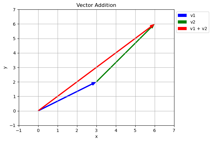

Magnitude: 3.605551275463989
Direction: 33.690067525979785 degrees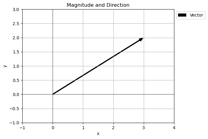

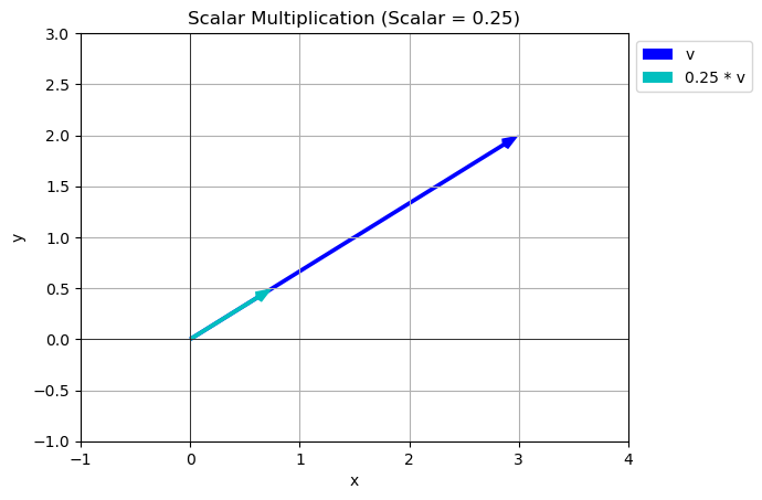
array([0.75, 0.5 ])

Span and Linear Dependence

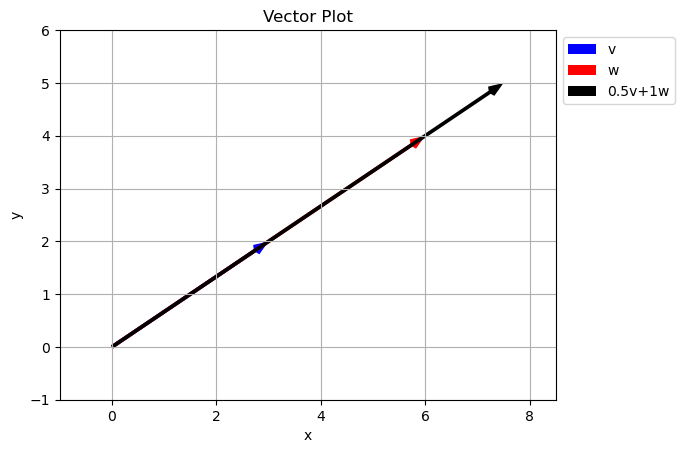
Last time we learned that we can both add two vectors together and multiply by a scalar. These two ideas actually give some interesting results. Given two vectors we can create a any third vector we want! (with some exceptions).

Let’s look at how this works:

v = np.array([3,2])
w = np.array([3,4])

avals = [-1.5,-1,-0.5,0.5,1,1.5]
bvals =[1]

for a in avals:
    for b in bvals:
        plot_vector(v,color='b',label='v')
        plot_vector(w,color='r',label='w')
        av = a*v
        bw = b*w
        combination = av+bw
        plot_vector(combination,color='k',label=f'{a}v+{b}w')
        plt.legend(loc='upper left', bbox_to_anchor=(1, 1))
        # Autoscale the axes based on the vectors
        all_x = [0, v[0], w[0], av[0], bw[0], combination[0]]
        all_y = [0, v[1], w[1], av[1], bw[1], combination[1]]
        min_x = min(all_x) - 1 
        max_x = max(all_x) + 1
        min_y = min(all_y) - 1
        max_y = max(all_y) + 1
        plt.xlim(min_x, max_x)
        plt.ylim(min_y, max_y)
        plt.show()
        
        

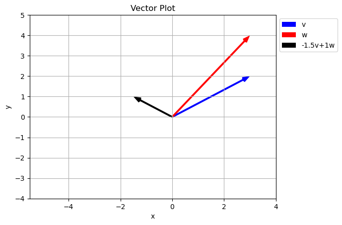
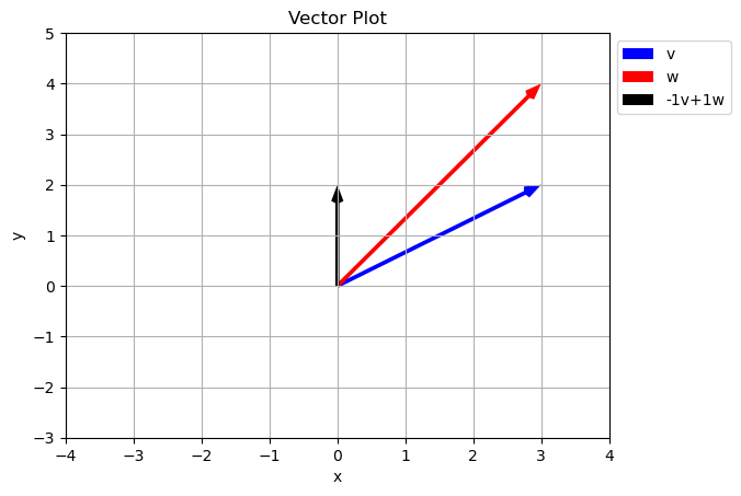
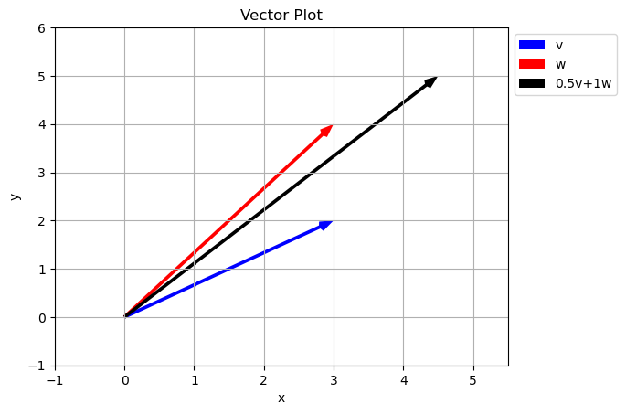
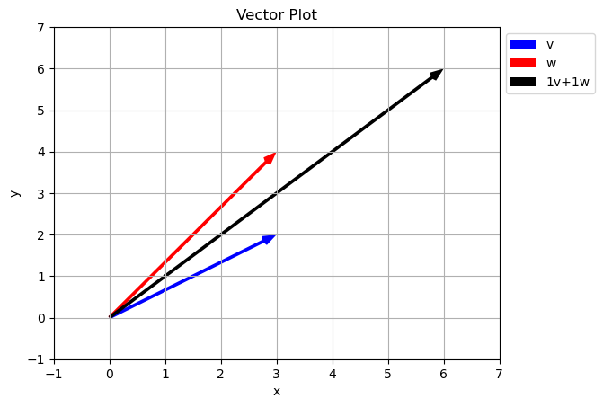
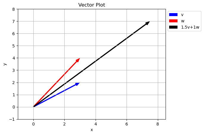
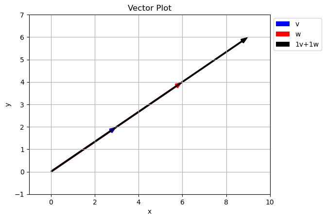
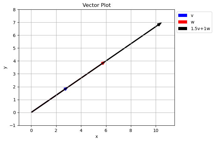
Notice how just by changing our scalar values we can reach any point in the \(xy\) plane. Is this true of any two vectors? Did we just get luck and pick special vectors?

Span of a set of vectors is the whole set of possible vectors that can be created by taking a linear combination of the vectors in the set.

Above, given the set of vectors:

\[\vec{v} = \begin{bmatrix} 3 \\ 2 \end{bmatrix}\]

\[\vec{w} = \begin{bmatrix} 3 \\ 4 \end{bmatrix}\]

what is the set of other vectors that can be created using \(a\vec{v}+b\vec{w}\) where \(a\) and \(b\) can be any real number? In the case above the span is the entire 2D plane.

Can we come up with an example where this fails?

\[\vec{v} = \begin{bmatrix} 3 \\ 2 \end{bmatrix}\]

\[\vec{w} = \begin{bmatrix} 6 \\ 4 \end{bmatrix}\]

v = np.array([3,2])
w = np.array([6,4])

avals = [-1.5,-1,-0.5,0.5,1,1.5]
bvals =[1]

for a in avals:
    for b in bvals:
        plot_vector(v,color='b',label='v')
        plot_vector(w,color='r',label='w')
        av = a*v
        bw = b*w
        combination = av+bw
        plot_vector(combination,color='k',label=f'{a}v+{b}w')
        plt.legend(loc='upper left', bbox_to_anchor=(1, 1))
        # Autoscale the axes based on the vectors
        all_x = [0, v[0], w[0], av[0], bw[0], combination[0]]
        all_y = [0, v[1], w[1], av[1], bw[1], combination[1]]
        min_x = min(all_x) - 1 
        max_x = max(all_x) + 1
        min_y = min(all_y) - 1
        max_y = max(all_y) + 1
        plt.xlim(min_x, max_x)
        plt.ylim(min_y, max_y)
        plt.show()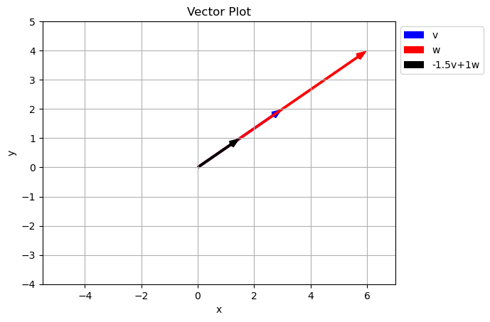

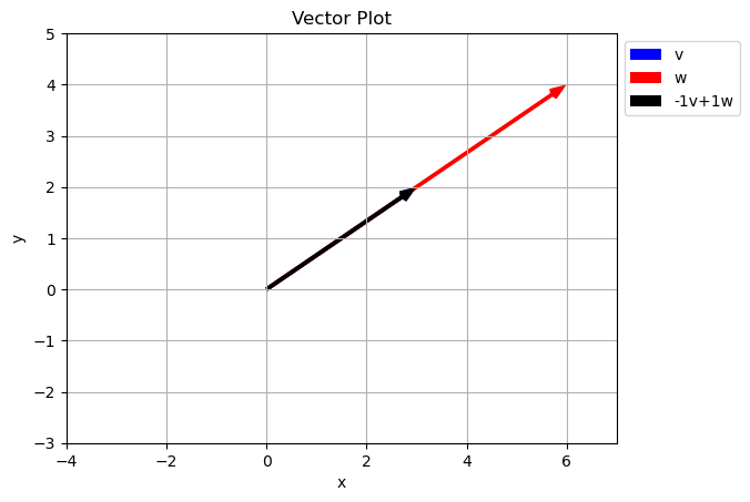
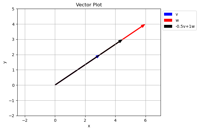
What happened here?

Because the two vectors in the original set with along the same line, we are unable to get any points off the line using just \(a\vec{v}+b\vec{w}\). In math this is called Linear Dependence

Two vectors are Linearly Independent if they do not lie along the same line. We can tell if two vectors are linearly dependent because one will be a scalar multiple of the other… they have different magnitudes but the same direction.

\[\vec{w} = \begin{bmatrix} 6 \\ 4 \end{bmatrix}=2\vec{v} = 2\begin{bmatrix} 3 \\ 2 \end{bmatrix}\]

You try

Which of the following vectors are linearly independent from \(\vec{v}\)

\[\vec{v} = \begin{bmatrix} 3 \\ 2 \end{bmatrix}\]

1. \[\vec{w_1} = \begin{bmatrix} -3 \\ 2 \end{bmatrix}\]
2. \[\vec{w_2} = \begin{bmatrix} 3/2 \\ 1 \end{bmatrix}\]
3. \[\vec{w_3} = \begin{bmatrix} 0 \\ 1 \end{bmatrix}\]

Linear Transformations and Basis Vectors

The idea of adding up linear combinations of vectors turns out to be REALLY IMPORTANT! This forms the logic behind linear transformations. We can use linear transformations to reshape and manipulate our data in ways that make predictions or patters much more obvious!

Basis Vectors

Basis vectors are the building blocks for transforming any vectors. They are the simplest vectors from which all other vectors can be built.

\[\hat{i} = \begin{bmatrix} 1 \\ 0 \end{bmatrix}\]

\[\hat{j} = \begin{bmatrix} 0 \\ 1 \end{bmatrix}\]

These two vectors are perpendicular to each other and both have a length of 1.

i_vec = np.array([1,0])
j_vec = np.array([0,1])

plot_vector(i_vec,color='r')
plot_vector(j_vec,color='b')
plt.xlim(-2,2)
plt.ylim(-2,2)
plt.axhline(0, color='black', linewidth=0.8)
plt.axvline(0, color='black', linewidth=0.8)
plt.show()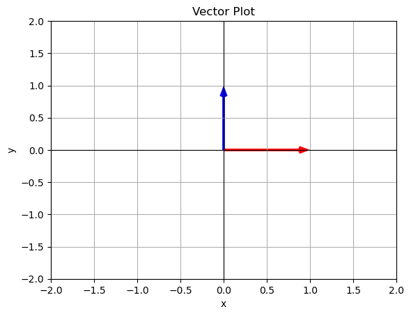

How can I create a new vector from these? Consider our good old fashioned vector:

\[\vec{v} = \begin{bmatrix} 3 \\ 2 \end{bmatrix}\]

I can write this as

\[\vec{v} = 3\hat{i}+2\hat{j} = 3\begin{bmatrix} 1 \\ 0 \end{bmatrix}+2\begin{bmatrix} 0 \\ 1 \end{bmatrix}=\begin{bmatrix} 3 \\ 0 \end{bmatrix}+\begin{bmatrix} 0 \\ 2 \end{bmatrix}=\begin{bmatrix} 3 \\ 2 \end{bmatrix}\]

Writing it in this way also emphasizes the fact that we go 3 steps in the \(x\) or \(\hat{i}\) direction and 2 steps in the \(y\) or \(\hat{j}\) direction.

You Try

Write each of the following vectors as a linear combination of basis vectors:

\[\hat{i} = \begin{bmatrix} 1 \\ 0 \end{bmatrix}\]

\[\hat{j} = \begin{bmatrix} 0 \\ 1 \end{bmatrix}\]

1. \[\vec{w_1} = \begin{bmatrix} -3 \\ 2 \end{bmatrix}\]
2. \[\vec{w_2} = \begin{bmatrix} 3/2 \\ 1 \end{bmatrix}\]
3. \[\vec{w_3} = \begin{bmatrix} 0 \\ 1 \end{bmatrix}\]

Matrices and Matrix Multiplication

A matrix is an array of numbers that all go together into rows and columns. For example we could have represented our basis vectors above as a matrix:

\[basis = \begin{bmatrix} 1& 0\\ 0& 1 \end{bmatrix}\]

In general a matrix can take any form and we usually use capital letters as a variable:

\[A = \begin{bmatrix} 2& -1&0\\ 0& 5&4 \end{bmatrix}\]

The dimensions of a matrix have to do with the number of rows and columns. We would say the matrix above is a “two by three” or \(2\times3\) matrix. Most of the time in applied linear algebra we will be dealing with square matrices - this just means it has the same number of rows and columns.

\[S = \begin{bmatrix} 4& 2&7\\ 5& 1&9\\ 4&0&1 \end{bmatrix}\]

this is a “three by three” matrix.

We can define matrix transformations using a matrix multiplication!

Example

Let’s say that we start with our original vectors and we want to rotate it 90 degrees.

\[\vec{v} = \begin{bmatrix} 3 \\ 2 \end{bmatrix}\]

We can apply the matrix

\[A = \begin{bmatrix} 0 & -1 \\ 1 & 0 \end{bmatrix}\]

This means we have to learn to calculate

\[A\cdot v = \begin{bmatrix} 0 & -1 \\ 1 & 0 \end{bmatrix}\begin{bmatrix} 3 \\ 2 \end{bmatrix}\]

This calculation is called a dot product and it is one form or matrix multiplication. What do we have to do?

Matrix Dot Product

\[\begin{bmatrix} a & b \\ c & d \end{bmatrix}\cdot\begin{bmatrix} x \\ y \end{bmatrix} = \begin{bmatrix} ax + by \\ cx + dy \end{bmatrix}\]

So in our example:

\[A\cdot v = \begin{bmatrix} 0 & -1 \\ 1 & 0 \end{bmatrix}\begin{bmatrix} 3 \\ 2 \end{bmatrix}=\begin{bmatrix} 0 + -2 \\ 3 + 0 \end{bmatrix}=\begin{bmatrix} -2 \\ 3 \end{bmatrix}\]

Lets look at a plot of these

v = np.array([3,2])
Av = np.array([-2,3])

plot_vector(v,color='r',label='v')
plot_vector(Av,color='b',label='Av')
plt.xlim(-3,3)
plt.ylim(-2,4)
plt.axhline(0, color='black', linewidth=0.8)
plt.axvline(0, color='black', linewidth=0.8)
plt.show()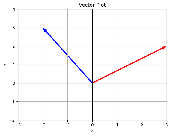

Calculating a dot product in Numpy

1. Enter the vector
2. Enter the matrix
3. Use np.matmul() to do the dot product

Most common error - shape mismatch! “mismatch in its core dimension” The inside dimensions must match when doing matrix dot products. Above we are multiplying a \(2\times2\) by a \(2\times1\). The first matrix has 2 columns to match up perfectly with the 2 rows of the second matrix.

# Calculating a dot product in Numpy
# Enter v
v = np.array([3,2])
v

array([3, 2])

# Enter the matrix
A = np.array([[0,-1],[1,0]])
A

array([[ 0, -1],
       [ 1,  0]])

# Do the dot product
v_rotate = np.matmul(A,v)
v_rotate

array([-2,  3])

## Here is the dot product in just one cell
v = np.array([3,2])
A = np.array([[0,-1],[1,0]])
v_new = np.matmul(A,v)
print(v,v_new)

[3 2] [-2  3]

Some Notes

You can also use .dot() and @ (shorthand for matmul) to do the dot product.

# Using the @ symbol
v_new_test = A@v
v_new_test

array([-2,  3])

Bigger Matrix Multiplications

We can apply the dot product or matrix multiplication to bigger matrices by following the same kind of pattern:

\[\begin{bmatrix} a & b \\ c & d \end{bmatrix}\begin{bmatrix} e& f \\ g&h \end{bmatrix} = \begin{bmatrix} ae+bg& af+bh \\ ce+dg& cf+dh \end{bmatrix} \]

notice how I am just doing the same thing… going across the rows of the first matrix and down the columns of the second matrix.

We can think of doing bigger matrix multiplications as combining transformations.

You Try

Do the following matrix multiplications first by hand then check your work with numpy.

1. \[\begin{bmatrix} 3&2 \\ 1&1 \end{bmatrix}\begin{bmatrix} -3 \\ 2 \end{bmatrix}\]
2. \[\begin{bmatrix} 0&1 \\ -1&0 \end{bmatrix}\begin{bmatrix} 3/2 \\ 1 \end{bmatrix}\]
3. \[\begin{bmatrix} 3&2 \\ 1&1 \end{bmatrix}\begin{bmatrix} 0&1 \\ -1&0 \end{bmatrix}\]

Where are we so far?

• We can define a vector
• We can use liner combinations of vectors to create new vectors
• We can do a matrix multiplication - dot product - which allows us to transform our vectors.

Matrix Identity

Whenever we are starting to do algebra with new objects it is important to think about identity elements. These are special matrices that although we do an operation, the result in unchanged. Think about adding zero or multiplying by 1.

For a matrix multiplying by 1 is multiplying by the identity matrix. In 2 dimensions this is given by

\[I=\begin{bmatrix} 1&0 \\ 0&1 \end{bmatrix}\]

It always has ones along the diagonal and zeros everywhere else. Let’s see the idenity in action:

\[I\cdot v = \begin{bmatrix} 1 & 0 \\ 0 & 1 \end{bmatrix}\begin{bmatrix} 3 \\ 2 \end{bmatrix}=\begin{bmatrix} 3 + 0 \\ 0 + 2 \end{bmatrix}=\begin{bmatrix} 3 \\ 2 \end{bmatrix}\]

Multiplying by the identity gave us back our vector.

Matrix Inverse

So how do we undo a transformation?

Above we found

\[A\cdot \vec{v}=\begin{bmatrix} -2 \\ 3 \end{bmatrix}\]

but what if we wanted to undo this multiplication, aka solve for \(\vec{v}\). Can we just divide?

\[\vec{v}=\frac{\begin{bmatrix} -2 \\ 3 \end{bmatrix}}{A}=\frac{\begin{bmatrix} -2 \\ 3 \end{bmatrix}}{\begin{bmatrix} 0 & -1 \\ 1 & 0 \end{bmatrix}} = nonsense\]

NO we cannot just divide by a matrix! With scalar values the inverse of multiplication is division:

\[ax = b \rightarrow x=\frac{b}{a}\]

When we are dealing with a matrix we need to find the matrix inverse:

\[A\vec{v} = \vec{b}\]

\[A^{-1}A\vec{v} = A^{-1}\vec{b}\]

\[\vec{v} = A^{-1}\vec{b}\]

\(A^{-1}\) is called the inverse of \(A\). One property of the inverse is that

\[A^{-1}A=I\]

It is possible to find the inverse by hand, but we wont do that in this class. We will use numpy.

A = np.array([[0,-1],[1,0]])
A

array([[ 0, -1],
       [ 1,  0]])

np.linalg.inv(A)

array([[ 0.,  1.],
       [-1., -0.]])

Let’s see if we get the identity if we multiply the inverse and A

np.linalg.inv(A)@A

array([[1., 0.],
       [0., 1.]])

Let’s see if we get back our \(\vec{v}\) if we multiply our \(\vec{v_{new}}\) and the inverse.

np.linalg.inv(A)@v_new

array([3., 2.])

Solving Systems of Equations

You can use the tools we have developed to solve systems of linear equations. Let’s look at this using an example.

Example 1

Say you want to solve for \(x\) and \(y\):

\[4x+2y=1\] \[3x-y=2\]

You probably can solve this with techniques learned in college algebra:

1. Sove the bottom equation for \(y\)

\[y = 3x-2\]

2. Sub this into the top equation

\[4x+2(3x-2) = 1\]

3. Solve for \(x\)

\[ x = \frac{1}{2} \]

4. Plug this in to solve for \(y\)

\[ y = \frac{-1}{2} \]

And this process while a bit boring is fine, until you want to solve lots of them or solve even bigger systems! Let’s do this the linear algebra way:

1. Write the equations in matrix form \(A\vec{x}=\vec{b}\)

let \(\vec{x} = \begin{bmatrix} x \\ y \end{bmatrix}\)

then we can write the equation

\[A\vec{x} = \begin{bmatrix} 4&2 \\ 3&-1 \end{bmatrix}\begin{bmatrix} x \\ y \end{bmatrix}=\begin{bmatrix} 1 \\ 2 \end{bmatrix}=\vec{b}\]

2. Solve using the matrix inverse:

if \(A\vec{x}=\vec{b}\) then \(\vec{x}=A^{-1}\vec{b}\)

A = np.array([[4,2],[3,-1]])
b = np.array([1,2])

x = np.linalg.inv(A)@b
x

array([ 0.5, -0.5])

We get the same result! \(x=\frac{1}{2}\) and \(y=\frac{-1}{2}\). The order matters here. Since x was in the top and y in the bottom we read the result in that order.

Example 2

Say you want to solve for \(x\), \(y\), and \(z\):

\[4x+2y+4z = 44\] \[5x+3y+7z = 56\] \[9x+3y+6z = 72\]

1. Write the system in matrix form

let \(\vec{x} = \begin{bmatrix} x \\ y \\ z \end{bmatrix}\)

\[\begin{bmatrix} 4&2&4 \\ 5&3&7 \\ 9&3&6 \end{bmatrix}\begin{bmatrix} x \\ y \\ z \end{bmatrix}=\begin{bmatrix} 44 \\ 56 \\ 72 \end{bmatrix}\]

A = np.array([[4,2,4],[5,3,7],[9,3,6]])
b = np.array([44,56,72])

x = np.linalg.inv(A)@b
x

array([ 2., 34., -8.])

So we find that \(x=2\), \(y=34\) and \(z=-8\). This is already WAY easier that doing all the substitutions!

A Brief Introduction to Linear Programming

Linear programming is a technique that every data science professional should be familiar with. This is a great old school method for optimizing systems subject to constraints. We will explore these ideas using an example.

Imagine that you own a company with two lines of products: the iPac and the iPac Ultra (iPacU). The iPac makes \$200 profit while the iPacU makes \$300 profit.

The assembly line one which these products are made can work for only 20 hours a day, and it takes 1 hours to make the iPac and 3 hours to make the iPacU.

Also, on the supply side only 45 production kits can be provided each day and it takes 6 kits to make an iPac with the iPacU requires 2 kits.

You always sell out of your supply, but the big question is how much of each product should we sell to maximize our profit?

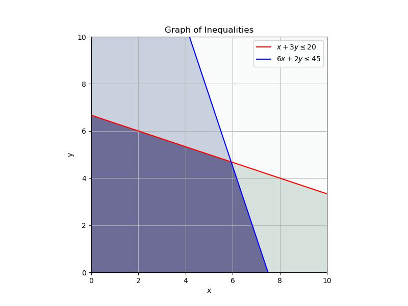
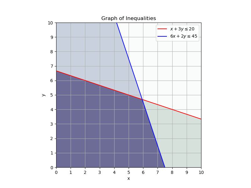
The first constraint in this system is the time - the fact that our assembly line can only run for 20 hours per day and it takes 1 hour to make iPac and 3 to make iPacU. Of course you would make more profit if you could run the factory for longer or make the products quicker. We can express this mathematically:

\[x+3y \leq 20\]

where we will let x represent the iPac and y represent the iPacU. This equation adds up the total number of hours we will spend making the products. Note that both \(x\) and \(y\) must be positive.

The second constraint in this system is supplies - the fact that we can only access 45 kits in a day and we need 6 to make the iPac and 2 to make the iPacU. Mathematically we can write:

\[6x+2y\leq 45\]

Here is a graph of the constraints with the less than area shaded in. The dark purple is the feasible region meaning that this is where the constraints are met.

INEQ Image

Next we want to maximize our profit. Mathematically:

\[Z = 200x+300y\]

So we are searching for a \(Z\) value that makes this line as far away from zero as possible. Here is a graph of a few \(Z\) values:

INEQ Image

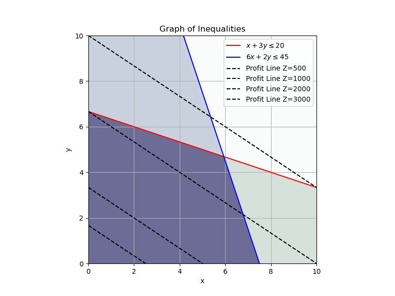
You can see that as we increase \(Z\) we get closer and closer to the point (corner) of the feasible region. Depending on the function we want to maximize, we may have to check more than one corner. In this case we can see what happens as \(Z\) increases.

So what do we need to do? First we need to solve the inequalities for where the maximum point is. Find the \(x\) and \(y\) values that solve:

\[x+3y = 20\] \[6x+2y = 45\]

or

\[\begin{bmatrix} 1&3 \\ 6&2 \end{bmatrix}\begin{bmatrix} x \\ y \end{bmatrix}=\begin{bmatrix} 20 \\ 45 \end{bmatrix}\]

we know how to do this!

# Graph the constraint lines

# Get the x values
x = np.linspace(0,10,1000)

# Solve them for y
y1 = (20-x)/3
y2 = (45-6*x)/2

plt.plot(x,y1,'b')
plt.plot(x,y2,'r')
plt.grid()
plt.xlim(0,10)
plt.ylim(0,10)
plt.show()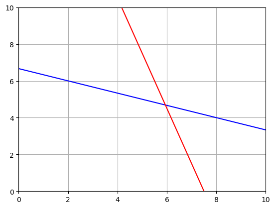

A = np.array([[1,3],[6,2]])
b = np.array([20,45])

x = np.linalg.inv(A)@b
print(x)

Z = 200*x[0]+300*x[1]
print(Z)

[5.9375 4.6875]
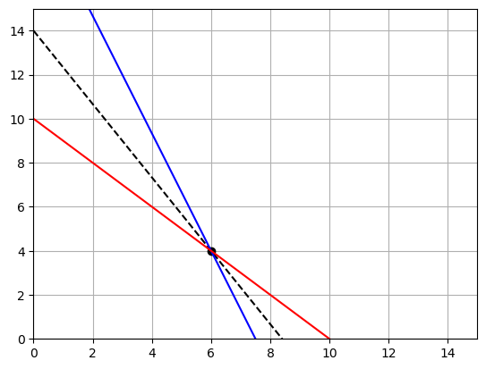
2593.75

# Add the point to the graph
# Add the profit to the graph

# Get the x values
x = np.linspace(0,10,1000)

# Solve them for y
y1 = (20-x)/3
y2 = (45-6*x)/2

plt.plot(x,y1,'b')
plt.plot(x,y2,'r')

# Add the point
plt.plot(5.9375,4.6875,'ok')

# Enter the max profit
Z = 2593.75
# Solve the profit equation for y
yp = (Z-200*x)/300
plt.plot(x,yp,'--k')

plt.grid()
plt.xlim(0,10)
plt.ylim(0,10)
plt.show()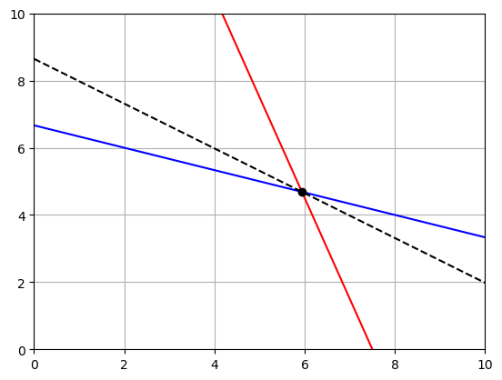

Interpret the results:

Our maximum profit will be \$2,593.75 when we make 5.9375 iPac and 4.6875 iPacU. Does it make sense to give numbers as decimals? Sometimes yes, but in this case not really. So what do we do?

We need to find the grid point closest to \((5.9375 4.6875)\) so we get whole numbers. We want to look for whole numbers on the constraint lines that are close to the point.

INEQ Image

Here we can see that the pint \((5 5)\) maximizes our profit while staying on the boundary of the constraints AND being a whole number. We should make 5 of each object!

NOTE you should check all possible intersection points. In this case we could also check the profit for the points \((0,20/3)\) and \((7.5,0)\). In the picture we can clearly see that we would have to move our profit line down to reach these points.

You Try

Maria has an online shop where she sells hand made paintings and cards.

It takes her 2 hours to complete 1 painting and 45 minutes to make a single card. She also has a day job and makes paintings and cards in her free time. She cannot spend more than 15 hours a week to make paintings and cards. Additionally, she should make not more than 10 paintings and cards per week.

She makes a profit of \$25 on painting and \$15 on each card. How many paintings and cards should she make each week to maximize her profit.

let \(x=\)painting and \(y\)=card

1. Write down a constraint on Maria’s time:

2. Write down a constraint on the number of objects Maria creates:

3. Write down the function for Maria’s profit - the thing you want to maximize

4. Graph the constraint lines

5. Write the system in matrix form

6. Use numpy to solve for the intersection point.

7. Plot the intersection point and the profit line to show that you have maximized the profit.

8. Interpret your results.

Joanna’s Solutions

\[2x+3/4y\leq 15\] \[x+y\leq 10\] \[Z = 25x+15y\]

# Graph the constraint lines

# Get the x values
x = np.linspace(0,10,1000)

# Solve them for y
y1 = 4*(15-2*x)/3
y2 = (10-x)

plt.plot(x,y1,'b')
plt.plot(x,y2,'r')
plt.grid()
plt.xlim(0,10)
plt.ylim(0,10)
plt.show()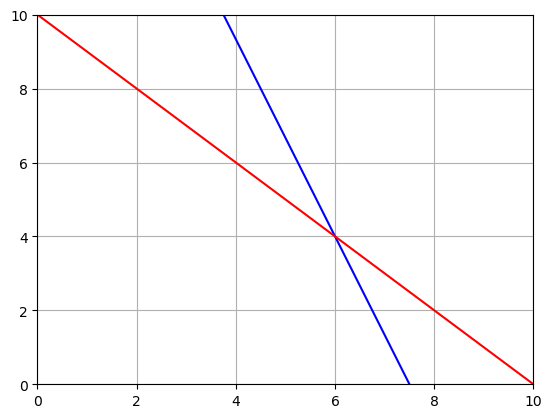

A = np.array([[2,3/4],[1,1]])
b = np.array([15,10])

x = np.linalg.inv(A)@b
print(x)

Z = 25*x[0]+15*x[1]
print(Z)

[6. 4.]
210.0

# Graph the constraint lines

# Get the x values
x = np.linspace(0,10,1000)

# Solve them for y
y1 = 4*(15-2*x)/3
y2 = (10-x)

# Add the point
plt.plot(6,4,'ok')

# Enter the max profit
Z = 210
# Solve the profit equation for y
yp = (Z-25*x)/15
plt.plot(x,yp,'--k')

plt.plot(x,y1,'b')
plt.plot(x,y2,'r')
plt.grid()
plt.xlim(0,15)
plt.ylim(0,15)
plt.show()