Math for Data Science

Important Information

Email: joanna_bieri@redlands.edu
Office Hours take place in Duke 209 unless otherwise noted – Office Hours Schedule

Today’s Goals:

Determinants
Eigenvalues
Applications

# We will just go ahead and import all the useful packages first.
import numpy as np
import sympy as sp
import pandas as pd
import matplotlib.pyplot as plt
from mpl_toolkits.mplot3d import Axes3D

# Special Functions 
from sklearn.metrics import r2_score, mean_squared_error
from sklearn.neighbors import KNeighborsClassifier
from scipy.stats import binom, beta, norm

# Functions to deal with dates
import datetime

# Code for plotting basis vectors
# You can just run this cell.
import matplotlib.patches as patches

def plot_basis_vectors_area(v1, v2):
    """
    Plots two basis vectors and the parallelogram they sweep out.
    """

    if len(v1) != 2 or len(v2) != 2:
        raise ValueError("Basis vectors must be 2-dimensional.")

    fig, ax = plt.subplots()

    # Set up the plot limits and aspect ratio
    max_val = max(abs(v1[0]), abs(v1[1]), abs(v2[0]), abs(v2[1]))
    ax.set_xlim(-max_val - 1, max_val + 1)
    ax.set_ylim(-max_val - 1, max_val + 1)
    # Make the grid look nice
    ax.set_aspect('equal', adjustable='box')
    ax.grid(True, linestyle='--', alpha=0.7)
    # Add the x and y axis
    ax.axhline(0, color='black', linewidth=0.5)
    ax.axvline(0, color='black', linewidth=0.5)
    # Labels
    ax.set_xlabel('x-axis')
    ax.set_ylabel('y-axis')
    # Title
    ax.set_title('Basis Vectors and Swept Area')

    # Plot the basis vectors
    ax.arrow(0, 0, v1[0], v1[1], head_width=0.2, head_length=0.3, fc='blue', ec='blue', label='Basis Vector 1')
    ax.arrow(0, 0, v2[0], v2[1], head_width=0.2, head_length=0.3, fc='green', ec='green', label='Basis Vector 2')

    # Calculate the vertices of the parallelogram
    origin = np.array([0, 0])
    p1 = v1
    p2 = v2
    p3 = v1 + v2
    # Plot the parallelogram
    polygon = patches.Polygon([origin, p1, p3, p2], closed=True, edgecolor='red', facecolor='red', alpha=0.3, label='Swept Area')
    ax.add_patch(polygon)

    ax.legend()
    plt.show()

    return abs(np.linalg.det(np.array([v1, v2])))

Vectors and Matrices (review)

Span of a set of vectors is the whole set of possible vectors that can be created by taking a linear combination of the vectors in the set.

Two vectors are Linearly Independent if they do not lie along the same line.

We can tell if two vectors are Linearly Dependent because one will be a scalar multiple of the other… they have different magnitudes but the same direction.

Matrix Dot Product

\[\begin{bmatrix} a & b \\ c & d \end{bmatrix}\cdot\begin{bmatrix} x \\ y \end{bmatrix} = \begin{bmatrix} ax + by \\ cx + dy \end{bmatrix}\]

\[\begin{bmatrix} a & b \\ c & d \end{bmatrix}\begin{bmatrix} e& f \\ g&h \end{bmatrix} = \begin{bmatrix} ae+bg& af+bh \\ ce+dg& cf+dh \end{bmatrix} \]

Using Numpy

v = np.array([3,2])
A = np.array([[0,-1],[1,0]])
v_new = np.matmul(A,v)
print(v,v_new)

Matrix Identity and Inverse

\[I=\begin{bmatrix} 1&0 \\ 0&1 \end{bmatrix}\]

\[A^{-1}A=I\]

np.linalg.inv(A)

Matrix Determinants

Remember from last time that we can use matrix multiplication to transform a vector. When we preform these linear transformations we often expand or squish our vector space. The amount of expansion or squishing can be helpful to know.

The determinant measures something about the size of a transformation. It measures how much a vector space changes when you apply a transformation. Are we squishing the vectors, expanding them, shearing them?

These also can be calculated by hand but we will use numpy in this class.

In two dimensions the determinant is give by

\[\begin{bmatrix} a&b \\ c&d \end{bmatrix}=a*d-b*c\]

We will consider the determinants of a few different matrices and see how they correspond to the transformations they represent.

Example 1

We will start by considering our basis vector and look at the are swept out.

\[\begin{bmatrix} 1&0 \\ 0&1 \end{bmatrix}\]

v1 = np.array([1,0])
v2 = np.array([0,1])
area = plot_basis_vectors_area(v1, v2)
print(f'The area in red is {area} square units')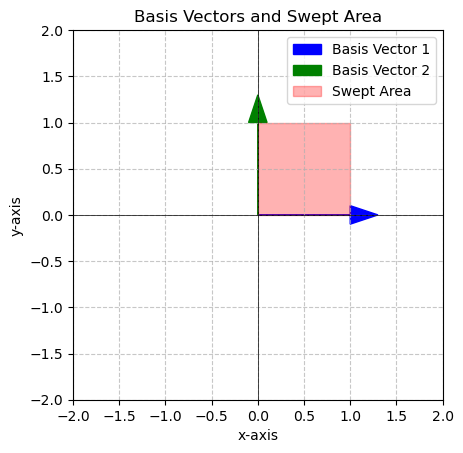

The area in red is 1.0 square units

Here we see that the area in red is 1 square unit. What happens if we apply a matrix multiplication?

\[\begin{bmatrix} 3&0 \\ 0&2 \end{bmatrix}\begin{bmatrix} 1&0 \\ 0&1 \end{bmatrix} = \begin{bmatrix} 3&0 \\ 0&2 \end{bmatrix}\]

v1 = np.array([3,0])
v2 = np.array([0,2])
area = plot_basis_vectors_area(v1, v2)
print(f'The area in red is {area} square units')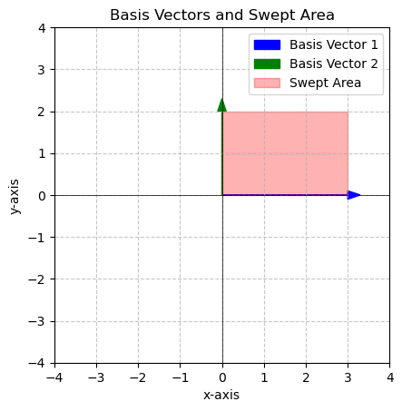

The area in red is 6.0 square units

Notice how the area changed. We expanded the length of both of our vectors this also expanded the space. How much was the space expanded?

Determinant

Consider the determinant of the matrix that defined our transformation

\[\begin{bmatrix} 3&0 \\ 0&2 \end{bmatrix} = 3*2-0*0=6\]

Notice that this is the exact amount that we expanded our vector space!

Example 2

Should a simple rotation change the area? Let’s see

Consider the rotation matrix from last time

\[\begin{bmatrix} 0&-1 \\ 1&0 \end{bmatrix}\]

Calculate the determinant by hand and compare to the numpy code below

A = np.array([[0,-1],[1,0]])
DET = np.linalg.det(A)
DET

1.0

This tells me that the overall area should not change if we apply this transformation. Let’s see this in practice.

\[\begin{bmatrix} 0&-1 \\ 1&0 \end{bmatrix}\begin{bmatrix} 3&0 \\ 0&2 \end{bmatrix}=\begin{bmatrix} 0&-2 \\ 3&0 \end{bmatrix}\]

v1 = np.array([0,-2])
v2 = np.array([3,0])
area = plot_basis_vectors_area(v1, v2)
print(f'The area in red is {area} square units')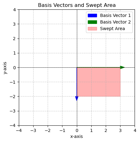

The area in red is 6.0 square units

The area did not change, but it was rotated to a new location!

You Try:

Starting with the following matrix

\[\begin{bmatrix} 1&1 \\ 1&-1 \end{bmatrix}\]

For each matrix multiplication below:

Find the determinant of the transformation given
Say in words what will happen to the area
Do the matrix multiplication to the the new matrix
Use the code to plot the new matrix and area.

\[\begin{bmatrix} 1&3 \\ 0&1 \end{bmatrix}\]

\[\begin{bmatrix} 1&0 \\ \frac{1}{2}&1 \end{bmatrix}\]

\[\begin{bmatrix} 1&3 \\ -2&1 \end{bmatrix}\]

\[\begin{bmatrix} 1&0.5 \\ 0.5&0.5 \end{bmatrix}\]

# Here is the plot of the original matrix
v1 = np.array([1,1])
v2 = np.array([1,-1])
area = plot_basis_vectors_area(v1, v2)
print(f'The area in red is {area} square units')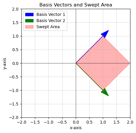

The area in red is 2.0 square units

# Your code here

# Your code here

# Your code here

# Your code here

Determinant of Linearly Dependent vectors

Consider the vectors:

\[\begin{bmatrix} 1 \\ 1 \end{bmatrix}\]

\[\begin{bmatrix} 4 \\ 4 \end{bmatrix}\]

First, how can you tell by looking that these vectors are linearly dependent?

Lets try to take the determinant of these two vectors:

\[\begin{bmatrix} 1&4 \\ 1&4 \end{bmatrix} = 1*4-1*4=0\]

What does this mean?

\[\begin{bmatrix} 1&4 \\ 1&4 \end{bmatrix} \begin{bmatrix} 1&1 \\ 1&-1 \end{bmatrix}= \begin{bmatrix} 5&-3 \\ 5&-3 \end{bmatrix}\]

v1 = np.array([5,5])
v2 = np.array([-3,-3])
area = plot_basis_vectors_area(v1, v2)
print(f'The area in red is {area} square units')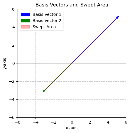

The area in red is 2.2204460492503135e-15 square units

Whenever two vectors are linearly dependent the determinant is zero! If we try to apply a transformation that has a zero determinant, the we are reducing our space to a single line. The area between the vectors is zero because they are on the same line!

Special Kinds of Matrices

Square

Equal number of rows and columns

\[\begin{bmatrix} 4&2&4 \\ 5&3&7 \\ 9&3&6 \end{bmatrix}\]

Identity

\[\begin{bmatrix} 1&0&0 \\ 0&1&0 \\ 0&0&1 \end{bmatrix}\]

Inverse

\[A = \begin{bmatrix} 4&2&4 \\ 5&3&7 \\ 9&3&6 \end{bmatrix}\]

\[A^{-1} = \begin{bmatrix} \frac{-1}{2}&0&\frac{1}{3} \\ \frac{11}{2}&-2&\frac{-4}{3} \\ -2&1&\frac{1}{3} \end{bmatrix}\]

A = np.array([[4,2,4],[5,3,7],[9,3,6]])
Ainv = np.array([[-1/2,0,1/3],[11/2,-2,-4/3],[-2,1,1/3]])

np.round(np.matmul(Ainv,A))

array([[ 1., -0., -0.],
       [ 0.,  1.,  0.],
       [-0., -0.,  1.]])

Diagonal

A diagonal matrix has values only along the diagonal and zeros everywhere else. Diagonal matrices are desirable in many computational settings because simplify the calculations.

\[A = \begin{bmatrix} 4&0&0 \\ 0&3&0 \\ 0&0&6 \end{bmatrix}\]

Triangular

Triangular matrices have non-zero values along the diagonal and non-zero values either above or below the diagonal with only zeros on the other side. They represent easy to solve systems and so are nice to work with.

Upper Triangular

\[A = \begin{bmatrix} 4&2&4 \\ 0&3&7 \\ 0&0&6 \end{bmatrix}\]

Lower Triangular

\[A = \begin{bmatrix} 4&0&0 \\ 5&3&0 \\ 9&3&6 \end{bmatrix}\]

Sparse Matrix

A sparse matrix is one that contains mostly zeros. From a computational standpoint the are very efficient since we don’t have to waste memory storing values that we know are zero.

\[A = \begin{bmatrix} 0&0&4 \\ 0&0&0 \\ 0&0&0 \end{bmatrix}\]

Eigenvalues and Eigenvectors

Eigenvalues and Eigenvectors are an important idea in applied linear algebra! The allow us to find the growth or decay rates in linear systems, construct solutions to systems, and to decompose matrices into basic components.

Eigenvalues and vectors are defined by the following equation

\[A\vec{v} = \lambda\vec{v}\]

Where \(\lambda\) is an eigenvalue and \(\vec{v}\) is an eigenvector. Notice what this equation is saying: Given a matrix \(A\) we are looking for a pair \(\vec{v}\) and \(\lambda\) such that when we multiply \(A\vec{v}\) we get back just a scalar multiple of \(\vec{v}\).

Let’s see this in action! Consider the matrix

\[A = \begin{bmatrix} 1&2\\ 4&5 \end{bmatrix}\]

we will use numpy to find eigenvalues

A = np.array([[1,2],[4,5]])
eigenvalues, eigenvectors = np.linalg.eig(A)

print("EIGENVALUES")
print(eigenvalues)

print("EIGENVECTORS")
print(eigenvectors)

EIGENVALUES
[-0.46410162  6.46410162]
EIGENVECTORS
[[-0.80689822 -0.34372377]
 [ 0.59069049 -0.9390708 ]]

Here we get two eigenvalues and two eigenvectors. THEY GO TOGETHER so we have

\[\lambda_1 = -0.4641016\;\;\; \vec{v_1} = \begin{bmatrix} -0.80689822 \\ 0.59069049 \end{bmatrix}\]

\[\lambda_2 = 6.46410162\;\;\; \vec{v_1} = \begin{bmatrix} -0.34372377\\ -0.9390708 \end{bmatrix}\]

Lets see what happens when we apply these to the equation that defines our eigenvalues and vectors

## A times v1
eigv =np.array([-0.80689822,0.59069049])
A = np.array([[1,2],[4,5]])

np.matmul(A,eigv)

array([ 0.37448276, -0.27414043])

# lambda1 times v2
lamb1 = -0.46410162
eigv =np.array([-0.80689822,0.59069049])
lamb1*eigv

array([ 0.37448277, -0.27414041])

Matrix Decomposition

Now what we can find eigenvalues and eigenvectors we can actually deconstruct \(A\) in an interesting way:

\[A = Q\Lambda Q^{-1}\]

where \(Q\) contains the eigenvectors and \(\Lambda\) has the eigenvalues on the diagonal. This is like factoring a matrix to make it easier to deal with. Let’s look at these objects

# Construct Q
Q = eigenvectors
Q

array([[-0.80689822, -0.34372377],
       [ 0.59069049, -0.9390708 ]])

# Construct Lambda Matrix
Lambda = np.array([[eigenvalues[0],0],[0,eigenvalues[1]]])
Lambda

array([[-0.46410162,  0.        ],
       [ 0.        ,  6.46410162]])

# Find the inverse Q^-1
Qinv = np.linalg.inv(Q)
Qinv

array([[-0.97741588,  0.35775904],
       [-0.61481016, -0.8398463 ]])

And we can check that this actually works!

Q@Lambda@Qinv

array([[1., 2.],
       [4., 5.]])

Summary

We now have the power to take determinants which help us test for linear dependence and tell us about the size of the transformation that we are applying to the vector space.

We can also find eigenvalues and eigenvectors and use these things to decompose a matrix system.

What’s next Now that we can calculate eigenvalues and eigenvectors we can sue these ideas to reduce the dimensionality of data and to transform our vectors space for better classification algorithms. This is what we will do next time!

You Try

Here are a few different matrix problems for you to practice with:

Are the following two vectors linearly dependent? Use the determinant test:

\[v1 = \begin{bmatrix} 2\\ 6 \end{bmatrix}\;\;\;v2 = \begin{bmatrix} 1\\ 3 \end{bmatrix}\]

Are the following two vectors linearly dependent? Use the determinant test:

\[v1 = \begin{bmatrix} 1\\ 2 \end{bmatrix} \;\;\; v2 = \begin{bmatrix} 1\\ 3 \end{bmatrix}\]

Consider the transformation given by the matrix

\[v1 = \begin{bmatrix} 1,2\\ 2,6 \end{bmatrix}\]

find the determinant and talk about the change in the area. Apply this transformation to the basis:

\[\begin{bmatrix} 1&1 \\ 1&-1 \end{bmatrix}\]

and plot your results.

Use linear algebra to solve the system of equations for \(x\),\(y\), and \(z\):

\[3x+1y+0z = 54\] \[2x+4y+1z=12\] \[3x+1y+8z=6\]

you will first need to write the system in matrix form.

Consider the matrix

\[\begin{bmatrix} 1&2 \\ 0&3 \end{bmatrix}\]

Find the eigenvalues and eigenvectors of this matrix. Write them as pairs \(\lambda_1,\;\;\vec{v_1}\) and \(\lambda_2,\;\;\vec{v_2}\)

Using the values you found in 5. write the system in decomposed form \[A = Q\Lambda Q^{-1}\] show values for \(Q\), \(Q^{-1}\) and \(\Lambda\).