# We will just go ahead and import all the useful packages first.
import numpy as np
import sympy as sp
import pandas as pd
import matplotlib.pyplot as plt
from mpl_toolkits.mplot3d import Axes3D

# Special Functions
from sklearn.metrics import r2_score, mean_squared_error
from sklearn.decomposition import PCA
from sklearn.preprocessing import StandardScaler
from scipy.stats import binom, beta, norm

# Functions to deal with dates
import datetimeMath for Data Science
Exam Review - Linear Algebra
Important Information
- Email: joanna_bieri@redlands.edu
- Office Hours take place in Duke 209 unless otherwise noted – Office Hours Schedule
Today’s Goals:
- Review topics from Probability for our Exam
Part 1
Matrix Computations:
Given the following definitions, complete each of the matrix computations:
\[a = 2,\;\;\; b=\frac{1}{4}, \;\;\; \vec{v}_1=\begin{bmatrix}1 \\ 1\end{bmatrix}, \;\;\;\vec{v}_2=\begin{bmatrix}2 \\ -2\end{bmatrix},\;\;\;\vec{v}_3=\begin{bmatrix}1 \\ -1\end{bmatrix}\]
\[A =\begin{bmatrix}1&2 \\ 3&1\end{bmatrix},\;\;\;B =\begin{bmatrix}1&2 \\ 0&1\end{bmatrix},\;\;\;C =\begin{bmatrix}0.5&1 \\ 0.5&2 \end{bmatrix},\;\;\;I =\begin{bmatrix}1&0 \\ 0&1\end{bmatrix}\]
- Calculate FIRST by hand and THEN using python:
\[a\vec{v}_1+b\vec{v}_3\]
Consider \(\vec{v}_1\),\(\vec{v}_2\),and \(\vec{v}_3\), which of these vectors are linearly dependent. How do you know?
Calculate FIRST by hand and THEN using python:
\[ A\cdot\vec{v}_1 \]
Find the determinants of \(A\),\(B\) and \(C\). What does this tell you about these matrices if we are thinking about the size of the transformation? Do these FIRST by hand then THEN using python.
In your head calculate \(I\cdot A\). Explain why this was easy enough to do in your head?
Find the eigenvalues and eigenvectors of \(A\), write down the pairs - the eigenvalue with it’s associated eigenvector. See if you can sketch the eigenvectors by hand.
a = 2
b = 1/4
v1 = np.array([1,1])
v2 = np.array([2,-2])
v3 = np.array([1,-1])

A = np.array([[1,2],[3,1]])
B = np.array([[1,2],[0,1]])
C = np.array([[1/2,1],[1/2,2]])
I = np.eye(2)

#1
v = a*v1+b*v3
print(v)

#2
if np.linalg.det(np.stack((v1,v2),axis=1)) == 0:
    print('v1 is linearly dependent to v2')
    print('They are constandt multiplues of each other')
    print('The determinant is zero!')
if np.linalg.det(np.stack((v2,v3),axis=1)) == 0:
    print('v2 is linearly dependent to v3')
    print('They are constandt multiplues of each other')
    print('The determinant is zero!')
if np.linalg.det(np.stack((v3,v1),axis=1)) == 0:
    print('v3 is linearly dependent to v1')
    print('They are constandt multiplues of each other')
    print('The determinant is zero!')

#3
print(A@v1)

#4
print(np.linalg.det(A))
print('This will expand our space - we dont care about the negative')
print(np.linalg.det(B))
print('This will not change the area')
print(np.linalg.det(C))
print('This will shrink our space.')

#5
print('I is the identity so multiplying A by it just gives us back A!')

#6
eigenvalues, eigenvectors = np.linalg.eig(A)
print("EIGENVALUES")
print(eigenvalues)

print("EIGENVECTORS")
print(eigenvectors)

print(f'lambda1 = {eigenvalues[0]} and v1 = {eigenvectors[:,0]}')
print(f'lambda2 = {eigenvalues[1]} and v2 = {eigenvectors[:,1]}')
[2.25 1.75]
v2 is linearly dependent to v3
They are constandt multiplues of each other
The determinant is zero!
[3 4]
-5.000000000000001
This will expand our space - we dont care about the negative
1.0
This will not change the area
0.5
This will shrink our space.
I is the identity so multiplying A by it just gives us back A!
EIGENVALUES
[ 3.44948974 -1.44948974]
EIGENVECTORS
[[ 0.63245553 -0.63245553]
[ 0.77459667 0.77459667]]
lambda1 = 3.4494897427831783 and v1 = [0.63245553 0.77459667]
lambda2 = -1.4494897427831779 and v2 = [-0.63245553 0.77459667]Part 2
Solving Linear Systems - Linear Programming
The annual Great Redlands Bake-Off Bonanza was just around the corner, and two best friends, Leo and Mia, were determined to win the coveted Golden Whisk trophy. They decided to specialize: Leo was a master of fluffy Cinnamon Swirl Buns, and Mia baked the most delectable Chocolate Chip Cookies in town. The two most critical limiting factors are their time and the number of presentation platters they have.
They have a total of 10 hours available for baking. - Each batch of Cinnamon Swirl Buns takes 3 hour to prepare and bake. - Each batch of Chocolate Chip Cookies takes 0.5 hours to prepare and bake.
They have only 12 presentation platters. - Each batch of Cinnamon Swirl Buns requires 2 platters. - Each batch of Chocolate Chip Cookies requires 1 platter.
Finally, they estimated their profit: - Each batch of Cinnamon Swirl Buns would earn them a profit of \$5. - Each batch of Chocolate Chip Cookies would earn them a profit of \$3.
Leo and Mia wanted to figure out how many batches of Cinnamon Swirl Buns and Chocolate Chip Cookies they should bake to maximize their total profit
Let
\(x\) = number of Cinnamon Swirl Buns
\(y\) = number of Chocolate Chip cookies
- Write down the constraints
- Write down the function you want to maximize
- Plot the feasible region
- Solve for the intersection point using the matrix inverse.
- Check the points and solve for the maximum profit.
# Constraint on time 3x+0.5y < 10
# Constraint on platters 2x+y < 12
# Profit Z = 5x+3y

x = np.linspace(0,5,100)

y1 = 2*(10-3*x)
y2 = 12-2*x

plt.plot(x,y1,'r')
plt.plot(x,y2,'b')
plt.grid()
plt.xlim(0,5)
plt.ylim(0,15)
plt.show()

print('The feasible area is below these lines but above x=0 and y=0')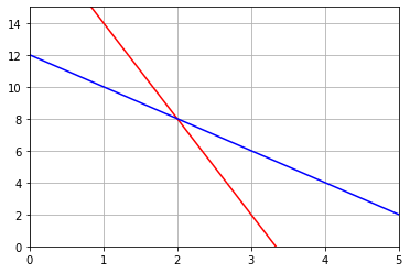
The feasible area is below these lines but above x=0 and y=0# Solve the intersection point
A = np.array([[3,0.5],[2,1]])
b = np.array([10,12])
x = np.linalg.inv(A)@b
print(x)
print('Max Profit at either (2,8), (10/3,0), or (0,12):')
print(5*x[0]+3*x[1])
print(5*(10/3)+3*0) # Where red line intersects y=0
print(5*0+3*12) # Where blue line intersects x=0[2. 8.]
Max Profit at either (2,8), (10/3,0), or (0,12):
34.0
16.666666666666668
36## 36 = 5x+3y
Z = 36
x = np.linspace(0,5,100)
y1 = 2*(10-3*x)
y2 = 12-2*x
plt.plot(x,y1,'r')
plt.plot(x,y2,'b')
plt.plot(x,(Z-5*x)/3,'-k')
plt.grid()
plt.show()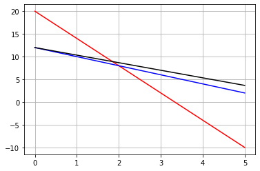
Part 3
Dimensionality Reduction:
Consider the data below with the following totally made up story:
You live in a magical dimension where crystals hold deep magic and allow the owner of the crystal great academic powers. Students who hold the magical crystals while studying have perfect retention of information and also gain a deep understanding of the applications of what they are learning. In fact, even after the crystal energy is drained, academic curiosity remains! The problem is that some crystals are not magical and instead cause an instant drain on energy. You can’t know just by looking what kind of crystal you are about to pick up. Since it is soon to be finals week we are going to set out to find only the best crystals for our academic pursuits!
- Read in the data and notice that there are four features and one label. What are the features and what is the label.
- Do a PCA analysis and project the data onto two dimensions and create a scatter plot.
- Report the Explained Variance Ratio and explain what it means.
- Now imagine that you find crystals (measured without picking them up of course) - You can load in the new crystals data. See if you can see where these new crystals land in the projected space - add them to your scatter plot. Which one would you keep? HINT You can use .transform() to run new data through your model!
Run the data through your standard scalar:
scalar.transform()Run the data through your PCA
PCA.transform()
filename='https://joannabieri.com/mathdatascience/data/glowcrystal.csv'
df = pd.read_csv(filename)
df| Radiant Intensity | Crystalline Volume | Aura Flux | Clarity Index | Magical | |
|---|---|---|---|---|---|
| 0 | 2.248357 | 11.620420 | 5.846293 | 80.751479 | 0.0 |
| 1 | 1.930868 | 8.074589 | 15.793547 | 81.039345 | 0.0 |
| 2 | 2.323844 | 6.615390 | 16.572855 | 77.959926 | 0.0 |
| 3 | 2.761515 | 13.058381 | 11.977227 | 80.696761 | 0.0 |
| 4 | 1.882923 | 15.154998 | 18.387143 | 80.879217 | 0.0 |
| ... | ... | ... | ... | ... | ... |
| 95 | 7.765849 | 35.149633 | 72.784599 | 93.123297 | 1.0 |
| 96 | 7.667538 | 46.297199 | 52.622988 | 88.147462 | 1.0 |
| 97 | 7.542670 | 42.151097 | 53.110435 | 100.415489 | 1.0 |
| 98 | 9.235818 | 45.690035 | 61.378669 | 94.541841 | 1.0 |
| 99 | 8.283487 | 44.407402 | 67.438634 | 99.951265 | 1.0 |
100 rows × 5 columns
features = ['Radiant Intensity','Crystalline Volume',' Aura Flux','Clarity Index']
color_mapping = [ 'mediumturquoise' if i == 1 else "yellowgreen" for i in df['Magical']]
df['color']=color_mapping
df| Radiant Intensity | Crystalline Volume | Aura Flux | Clarity Index | Magical | color | |
|---|---|---|---|---|---|---|
| 0 | 2.248357 | 11.620420 | 5.846293 | 80.751479 | 0.0 | yellowgreen |
| 1 | 1.930868 | 8.074589 | 15.793547 | 81.039345 | 0.0 | yellowgreen |
| 2 | 2.323844 | 6.615390 | 16.572855 | 77.959926 | 0.0 | yellowgreen |
| 3 | 2.761515 | 13.058381 | 11.977227 | 80.696761 | 0.0 | yellowgreen |
| 4 | 1.882923 | 15.154998 | 18.387143 | 80.879217 | 0.0 | yellowgreen |
| ... | ... | ... | ... | ... | ... | ... |
| 95 | 7.765849 | 35.149633 | 72.784599 | 93.123297 | 1.0 | mediumturquoise |
| 96 | 7.667538 | 46.297199 | 52.622988 | 88.147462 | 1.0 | mediumturquoise |
| 97 | 7.542670 | 42.151097 | 53.110435 | 100.415489 | 1.0 | mediumturquoise |
| 98 | 9.235818 | 45.690035 | 61.378669 | 94.541841 | 1.0 | mediumturquoise |
| 99 | 8.283487 | 44.407402 | 67.438634 | 99.951265 | 1.0 | mediumturquoise |
100 rows × 6 columns
np.random.seed(42)  # for reproducibility

# Select the features - CHANGE BASED ON YOUR DATA
features = ['Radiant Intensity','Crystalline Volume',' Aura Flux','Clarity Index']
# Normalize the data
# Z-score normalization
scalar = StandardScaler()
inputs = scalar.fit_transform(df[features]) #CHANGE BASED ON YOUR DATA

# Create the model
model = PCA(n_components=2) #CHANGE BASED ON NUMBER OF COMPONENTS YOU WANT
x_proj = model.fit_transform(inputs)

# Make a scatter plot
plt.figure(figsize=(8, 6))  # Adjust figure size as needed
# Color the plot based on malignant or not
color = df['color'].values
plt.scatter(x_proj[:,0], x_proj[:,1], c=color) #plot points
plt.xlabel("Data Projected onto 2D")
plt.axhline(0, color='black', linewidth=0.8) #draw the numberline
plt.grid(True, axis='x', linestyle='--', alpha=0.6) #add grid for x-axis
plt.show()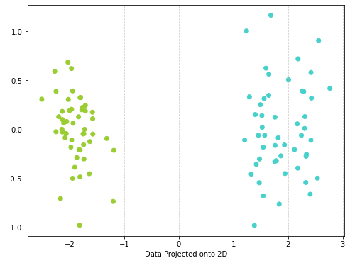
new_crystals = np.array([[2,    11.5,   5.8,     81],
                           [1.8,    15, 18.3,   90],
                           [7.5,    42, 54, 95]])

new_crystals_df = pd.DataFrame(new_crystals, columns=features)
print("\nNew Crystals Data:")
print(new_crystals_df)

new_inputs = scalar.transform(new_crystals_df[features])
new_x_proj = model.transform(new_inputs)
print(new_x_proj)
New Crystals Data:
   Radiant Intensity  Crystalline Volume   Aura Flux  Clarity Index
0                2.0                11.5         5.8           81.0
1                1.8                15.0        18.3           90.0
2                7.5                42.0        54.0           95.0
[[-2.02738704  0.15560347]
 [-1.19472878 -0.4876404 ]
 [ 1.50526909  0.2907625 ]]
# Make a scatter plot
plt.figure(figsize=(8, 6)) # Adjust figure size as needed
# Color the plot based on malignant or not
color = df['color'].values
plt.scatter(x_proj[:,0], x_proj[:,1], c=color) #plot points
plt.scatter(new_x_proj[:,0], new_x_proj[:,1], c='red') #plot points
plt.xlabel("Data Projected onto 2D")
plt.axhline(0, color='black', linewidth=0.8) #draw the numberline
plt.grid(True, axis='x', linestyle='--', alpha=0.6) #add grid for x-axis
plt.show()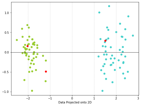
I would take the third crystal!!!